Descriptive statistics

---

We will use the RSiena objects of clubs to describe the kudos networks, constant covariates and behavioral variables.

Getting started

Clean the working environment and load in the club data.

# clean the working environment 
rm (list = ls( ))

# load the RSiena objects
load("clubdata_rsiena_freq.RData")
load("clubdata_rsiena_vol.RData")

# and the list containing club data-setes
load("clubdata.RData")

general custom functions

• fpackage.check: Check if packages are installed (and install if not) in R (source)
• fload.R: function to load R-objects under new names.

fpackage.check <- function(packages) {
    lapply(packages, FUN = function(x) {
        if (!require(x, character.only = TRUE)) {
            install.packages(x, dependencies = TRUE)
            library(x, character.only = TRUE)
        }
    })
}

fload.R  <- function(fileName){
  load(fileName)
  get(ls()[ls() != "fileName"])
}

necessary packages

We install and load the packages we need later on:

• RSiena: RSiena models, some descriptives on network level
• igraph: Descriptives (dyad/triad census, degrees)
• tidyverse
• tidyr: for tidy data
• moments: for calculating statistics (e.g., kurtosis, standard error)
• dplyr: for data manipulation
• ggplot2: for data visualization
• forcats: for handling categorical variabl
• knitr: for generating tables
• kableExtra: for manipulating tables
• network: for network analysis
• sna: for network analysis

packages = c("RSiena", "igraph", "tidyverse", "tidyr", "moments", "dplyr", "ggplot2", "forcats", "knitr", "kableExtra", "network", "sna")

fpackage.check(packages)

additional functions

Now define some additional functions we use later on to describe our data (see www.jochemtolsma.nl).

• fdensity: calculate density (exclude NA and structural zeros)
  
• fdensityintra: calculate density within group (exclude NA and structural zeros)
  
• fdensityinter: calculate density between groups (exclude NA and structural zeros)
  
• fhomomat: based on ego/alter characteristics, construct dyad characteristic whether or not ego/alter are same
• fndyads: calculate all valid dyads (no NA or structural zeros)
  
• fscolnet: calculate Coleman’s segregation index on the network-level
  
• fMoran.i: calculate Moran’s I spatial autocorrelation statistic (see here)

# density: observed relations divided by possible relations
fdensity <- function(x) {
    # x is your nomination network make sure diagonal cells are NA
    diag(x) <- NA
    # take care of RSiena structural zeros, set as missing.
    x[x == 10] <- NA
    sum(x == 1, na.rm = T)/(sum(x == 1 | x == 0, na.rm = T))
}

# calculate intragroup density
fdensityintra <- function(x, A) {
    # A is matrix indicating whether nodes in dyad have same node attributes
    diag(x) <- NA
    x[x == 10] <- NA
    diag(A) <- NA
    sum(x == 1 & A == 1, na.rm = T)/(sum((x == 1 | x == 0) & A == 1, na.rm = T))
}

# calculate intragroup density
fdensityinter <- function(x, A) {
    # A is matrix indicating whether nodes in dyad have same node attributes
    diag(x) <- NA
    x[x == 10] <- NA
    diag(A) <- NA
    sum(x == 1 & A != 1, na.rm = T)/(sum((x == 1 | x == 0) & A != 1, na.rm = T))
}

# construct dyad characteristic whether nodes are similar/homogenous
fhomomat <- function(x) {
    # x is a vector of node-covariate
    xmat <- matrix(x, nrow = length(x), ncol = length(x))
    xmatt <- t(xmat)
    xhomo <- xmat == xmatt
    return(xhomo)
}

# a function to calculate all valid dyads.
fndyads <- function(x) {
    diag(x) <- NA
    x[x == 10] <- NA
    (sum((x == 1 | x == 0), na.rm = T))
}

# a function to calculate all valid intragroupdyads.
fndyads2 <- function(x, A) {
    diag(x) <- NA
    x[x == 10] <- NA
    diag(A) <- NA
    (sum((x == 1 | x == 0) & A == 1, na.rm = T))
}


fscolnet <- function(network, ccovar) {
    # Calculate coleman on network level:
    # https://reader.elsevier.com/reader/sd/pii/S0378873314000239?token=A42F99FF6E2B750436DD2CB0DB7B1F41BDEC16052A45683C02644DAF88215A3379636B2AA197B65941D6373E9E2EE413
    
    fhomomat <- function(x) {
        xmat <- matrix(x, nrow = length(x), ncol = length(x))
        xmatt <- t(xmat)
        xhomo <- xmat == xmatt
        return(xhomo)
    }
    
    fsumintra <- function(x, A) {
        # A is matrix indicating whether nodes constituting dyad have same characteristics
        diag(x) <- NA
        x[x == 10] <- NA
        diag(A) <- NA
        sum(x == 1 & A == 1, na.rm = T)
    }
    
    # expecation w*=sum_g sum_i (ni((ng-1)/(N-1)))
    network[network == 10] <- NA
    ni <- rowSums(network, na.rm = T)
    ng <- NA
    for (i in 1:length(ccovar)) {
        ng[i] <- table(ccovar)[rownames(table(ccovar)) == ccovar[i]]
    }
    N <- length(ccovar)
    wexp <- sum(ni * ((ng - 1)/(N - 1)), na.rm = T)
    
    # wgg1 how many intragroup ties
    w <- fsumintra(network, fhomomat(ccovar))
    
    Scol_net <- ifelse(w >= wexp, (w - wexp)/(sum(ni, na.rm = T) - wexp), (w - wexp)/wexp)
    return(Scol_net)
}

fMoran.I <- function(x, weight, scaled = FALSE, na.rm = FALSE, alternative = "two.sided", rowstandardize = TRUE) {
    if (rowstandardize) {
        if (dim(weight)[1] != dim(weight)[2]) 
            stop("'weight' must be a square matrix")
        n <- length(x)
        if (dim(weight)[1] != n) 
            stop("'weight' must have as many rows as observations in 'x'")
        ei <- -1/(n - 1)
        nas <- is.na(x)
        if (any(nas)) {
            if (na.rm) {
                x <- x[!nas]
                n <- length(x)
                weight <- weight[!nas, !nas]
            } else {
                warning("'x' has missing values: maybe you wanted to set na.rm = TRUE?")
                return(list(observed = NA, expected = ei, sd = NA, p.value = NA))
            }
        }
        ROWSUM <- rowSums(weight)
        ROWSUM[ROWSUM == 0] <- 1
        weight <- weight/ROWSUM
        s <- sum(weight)
        m <- mean(x)
        y <- x - m
        cv <- sum(weight * y %o% y)
        v <- sum(y^2)
        obs <- (n/s) * (cv/v)
        if (scaled) {
            i.max <- (n/s) * (sd(rowSums(weight) * y)/sqrt(v/(n - 1)))
            obs <- obs/i.max
        }
        S1 <- 0.5 * sum((weight + t(weight))^2)
        S2 <- sum((apply(weight, 1, sum) + apply(weight, 2, sum))^2)
        s.sq <- s^2
        k <- (sum(y^4)/n)/(v/n)^2
        sdi <- sqrt((n * ((n^2 - 3 * n + 3) * S1 - n * S2 + 3 * s.sq) - k * (n * (n - 1) * S1 - 2 * n * 
            S2 + 6 * s.sq))/((n - 1) * (n - 2) * (n - 3) * s.sq) - 1/((n - 1)^2))
        alternative <- match.arg(alternative, c("two.sided", "less", "greater"))
        pv <- pnorm(obs, mean = ei, sd = sdi)
        if (alternative == "two.sided") 
            pv <- if (obs <= ei) 
                2 * pv else 2 * (1 - pv)
        if (alternative == "greater") 
            pv <- 1 - pv
        list(observed = obs, expected = ei, sd = sdi, p.value = pv)
    } else {
        if (dim(weight)[1] != dim(weight)[2]) 
            stop("'weight' must be a square matrix")
        n <- length(x)
        if (dim(weight)[1] != n) 
            stop("'weight' must have as many rows as observations in 'x'")
        ei <- -1/(n - 1)
        nas <- is.na(x)
        if (any(nas)) {
            if (na.rm) {
                x <- x[!nas]
                n <- length(x)
                weight <- weight[!nas, !nas]
            } else {
                warning("'x' has missing values: maybe you wanted to set na.rm = TRUE?")
                return(list(observed = NA, expected = ei, sd = NA, p.value = NA))
            }
        }
        # ROWSUM <- rowSums(weight) ROWSUM[ROWSUM == 0] <- 1 weight <- weight/ROWSUM
        s <- sum(weight)
        m <- mean(x)
        y <- x - m
        cv <- sum(weight * y %o% y)
        v <- sum(y^2)
        obs <- (n/s) * (cv/v)
        if (scaled) {
            i.max <- (n/s) * (sd(rowSums(weight) * y)/sqrt(v/(n - 1)))
            obs <- obs/i.max
        }
        S1 <- 0.5 * sum((weight + t(weight))^2)
        S2 <- sum((apply(weight, 1, sum) + apply(weight, 2, sum))^2)
        s.sq <- s^2
        k <- (sum(y^4)/n)/(v/n)^2
        sdi <- sqrt((n * ((n^2 - 3 * n + 3) * S1 - n * S2 + 3 * s.sq) - k * (n * (n - 1) * S1 - 2 * n * 
            S2 + 6 * s.sq))/((n - 1) * (n - 2) * (n - 3) * s.sq) - 1/((n - 1)^2))
        alternative <- match.arg(alternative, c("two.sided", "less", "greater"))
        pv <- pnorm(obs, mean = ei, sd = sdi)
        if (alternative == "two.sided") 
            pv <- if (obs <= ei) 
                2 * pv else 2 * (1 - pv)
        if (alternative == "greater") 
            pv <- 1 - pv
        list(observed = obs, expected = ei, sd = sdi, p.value = pv)
    }
    
    
}

---

We cover the following:

• club characteristics
• network structure in Kudos networks
• gender composition / segregation
• behavior: activity level (frequency and duration) and correlation
• spatial network autocorrelation: behavioral similarity in networks

---

Print report

Make sure to check the output of the ‘print01Report()’ function for general data descripton (degrees, network size, etc.) and a general overview of the dataset. Output is printed in a .txt file in the directory specified.

Club 1

df <- clubdata_rsiena_freq[[1]] # grab club 
print01Report(df, modelname="files/club1")

Club 2

df <- clubdata_rsiena_freq[[2]] # grab club 
print01Report(df, modelname="files/club2")

Club 3

df <- clubdata_rsiena_freq[[3]] # grab club 
print01Report(df, modelname="files/club3")

Club 4

df <- clubdata_rsiena_freq[[4]] # grab club 
print01Report(df, modelname="files/club4")

Club 5

df <- clubdata_rsiena_freq[[5]] # grab club 
print01Report(df, modelname="files/club5")

---

Club characteristics

Some club characteristics. We show the size of the network (the number of actors) for each club and the number of active members currently (18-1-2021) on Strava, by adding to www.strava.com/clubs/… the original club id.

# attrieve from the clubdata the number of actors in each network
netsize <- c( 
  length(clubdata_rsiena_freq[[1]]$nodeSets$Actors), 
  length(clubdata_rsiena_freq[[2]]$nodeSets$Actors), 
  length(clubdata_rsiena_freq[[3]]$nodeSets$Actors), 
  length(clubdata_rsiena_freq[[4]]$nodeSets$Actors), 
  length(clubdata_rsiena_freq[[5]]$nodeSets$Actors)) 

clubsize <- c(66, 127, 373, 15, 169) # find the number of members currently on Strava

df <- data.frame( netsize = netsize, clubsize = clubsize )

print(df)

#>   netsize clubsize
#> 1      27       66
#> 2      58      127
#> 3     159      373
#> 4       9       15
#> 5      76      169

---

Kudos network

Now let’s describe the Kudos network.

1. Node-level

Starting, again, with indegrees and outdegrees: who receives and gives Kudos? We take from the RSiena object the Kudos network for each club, subset the first wave, and turn it into an igraph object.

Club 1

df <- clubdata_rsiena_freq[[1]] # grab club 
knet <- df$depvars$kudonet # take Kudo network
knet1 <- knet[,,1] # take wave 1 only for now

# make an 'igraph object'
G1 <- igraph::graph_from_adjacency_matrix(knet1, mode = "directed", weighted = NULL, diag = TRUE, add.colnames = NA, add.rownames = NA)

# find in- and outdegree for each node
hist(igraph::degree(G1, mode="out"), xlab="outdegree", main="histogram of Kudo outdegree")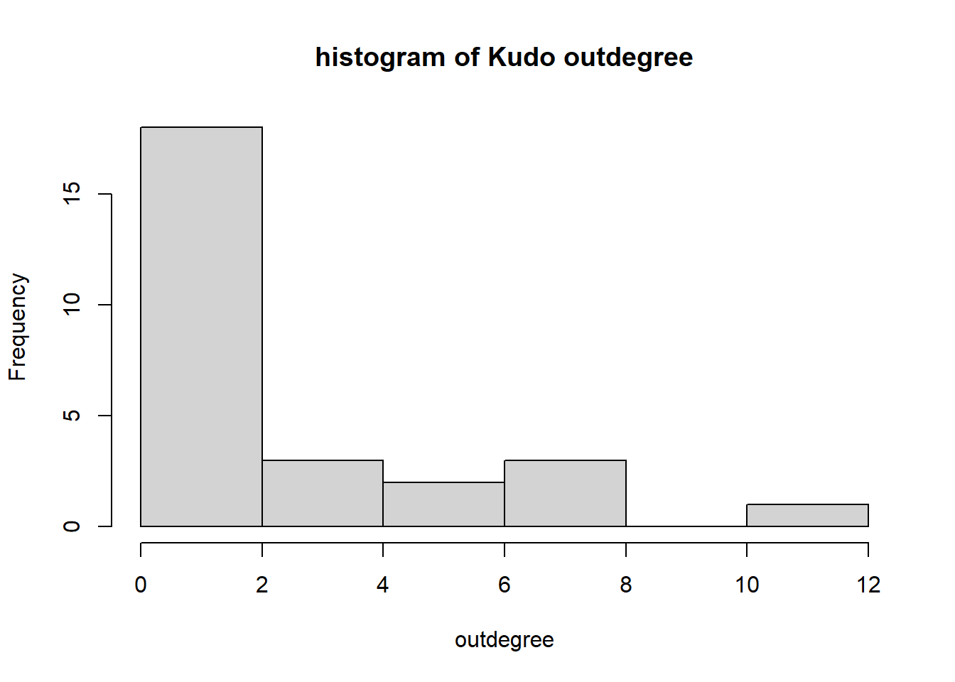

hist(igraph::degree(G1, mode="in"), xlab="indegree", main="histogram of Kudo indegree")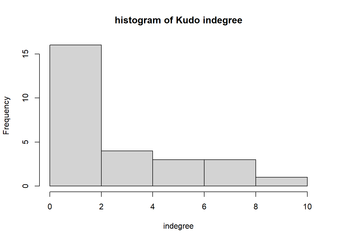

Club 2

df <- clubdata_rsiena_freq[[2]] # grab club t
knet <- df$depvars$kudonet # take Kudo network
knet1 <- knet[,,1] # take wave 1 only for now

# make an 'igraph object'
G1 <- igraph::graph_from_adjacency_matrix(knet1, mode = "directed", weighted = NULL, diag = TRUE, add.colnames = NA, add.rownames = NA)

# find in- and outdegree for each node
hist(igraph::degree(G1, mode="out"), xlab="outdegree", main="histogram of Kudo outdegree")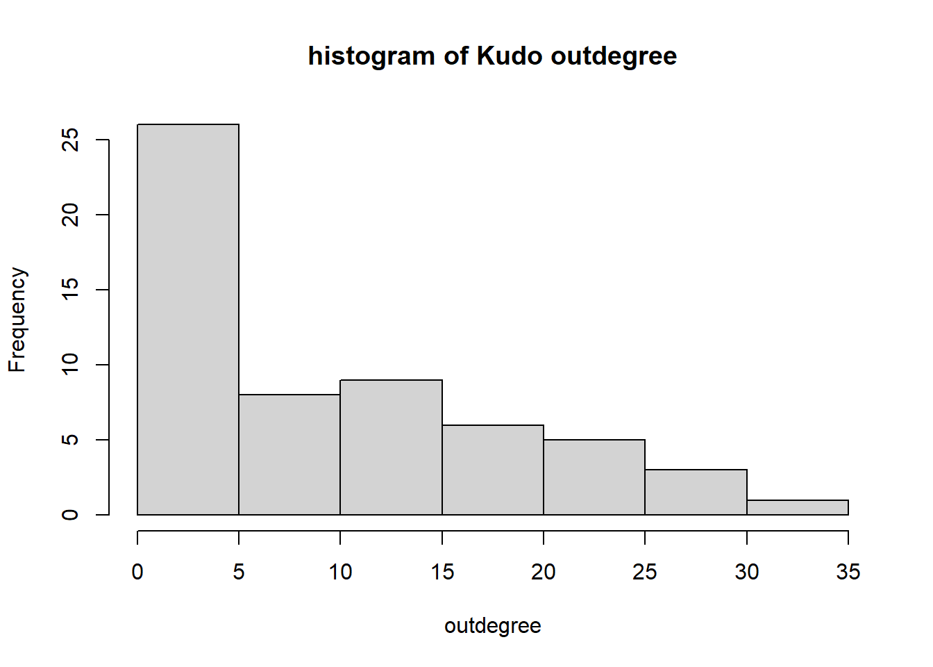

hist(igraph::degree(G1, mode="in"), xlab="indegree", main="histogram of Kudo indegree")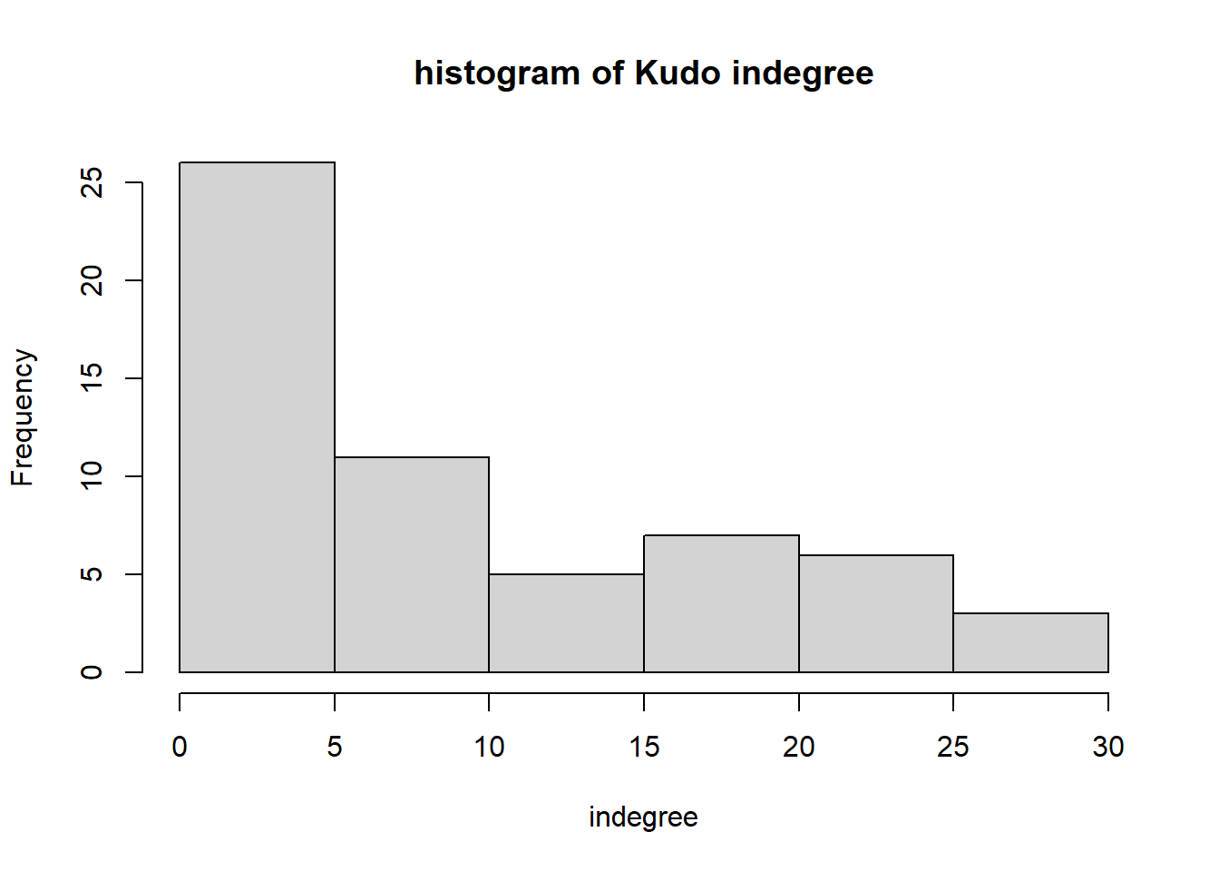

Club 3

df <- clubdata_rsiena_freq[[3]] # grab club 
knet <- df$depvars$kudonet # take Kudo network
knet1 <- knet[,,1] # take wave 1 only for now

# make an 'igraph object'
G1 <- igraph::graph_from_adjacency_matrix(knet1, mode = "directed", weighted = NULL, diag = TRUE, add.colnames = NA, add.rownames = NA)

# find in- and outdegree for each node
hist(igraph::degree(G1, mode="out"), xlab="outdegree", main="histogram of Kudo outdegree")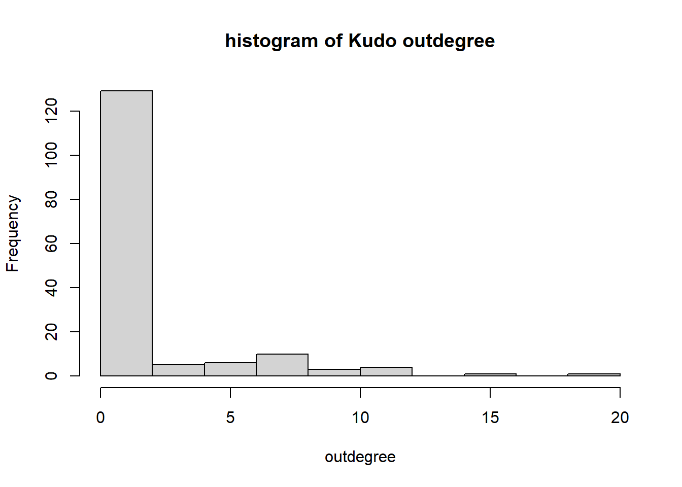

hist(igraph::degree(G1, mode="in"), xlab="indegree", main="histogram of Kudo indegree")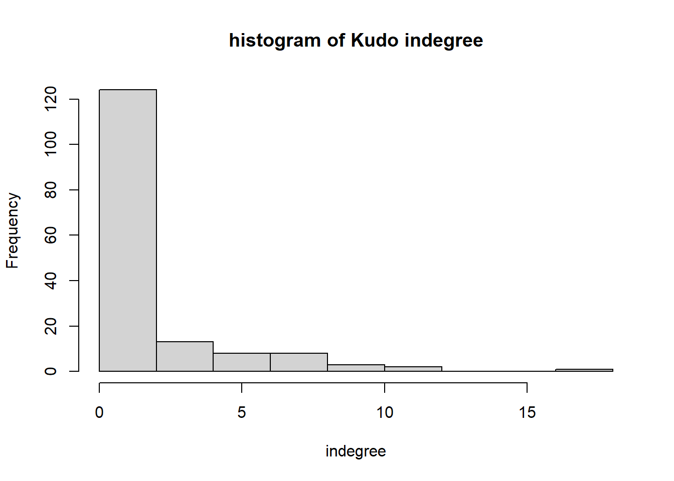

Club 4

df <- clubdata_rsiena_freq[[4]] # grab club 
knet <- df$depvars$kudonet # take Kudo network
knet1 <- knet[,,1] # take wave 1 only for now

# make an 'igraph object'
G1 <- igraph::graph_from_adjacency_matrix(knet1, mode = "directed", weighted = NULL, diag = TRUE, add.colnames = NA, add.rownames = NA)

# find in- and outdegree for each node
hist(igraph::degree(G1, mode="out"), xlab="outdegree", main="histogram of Kudo outdegree")

hist(igraph::degree(G1, mode="in"), xlab="indegree", main="histogram of Kudo indegree")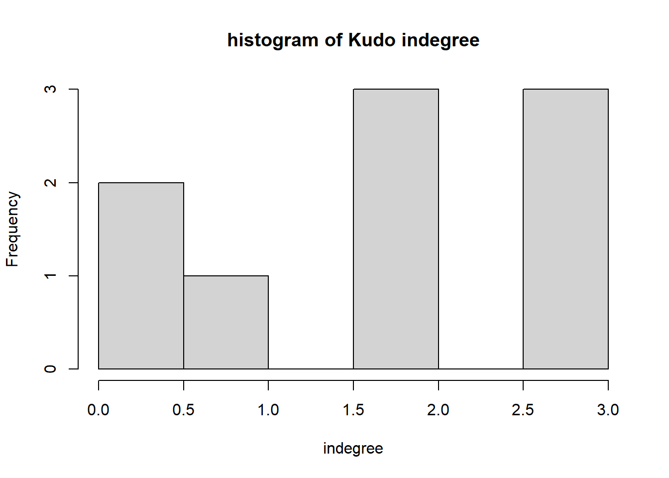

Club 5

df <- clubdata_rsiena_freq[[5]] # grab club 
knet <- df$depvars$kudonet # take Kudo network
knet1 <- knet[,,1] # take wave 1 only for now

# make an 'igraph object'
G1 <- igraph::graph_from_adjacency_matrix(knet1, mode = "directed", weighted = NULL, diag = TRUE, add.colnames = NA, add.rownames = NA)

# find in- and outdegree for each node
hist(igraph::degree(G1, mode="out"), xlab="outdegree", main="histogram of Kudo outdegree")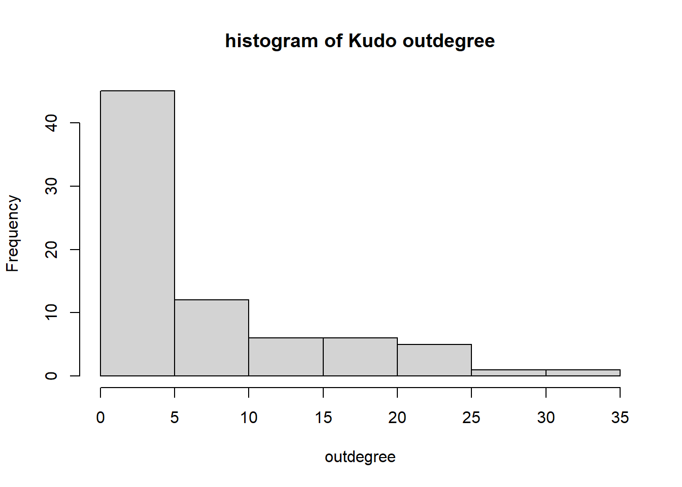

hist(igraph::degree(G1, mode="in"), xlab="indegree", main="histogram of Kudo indegree")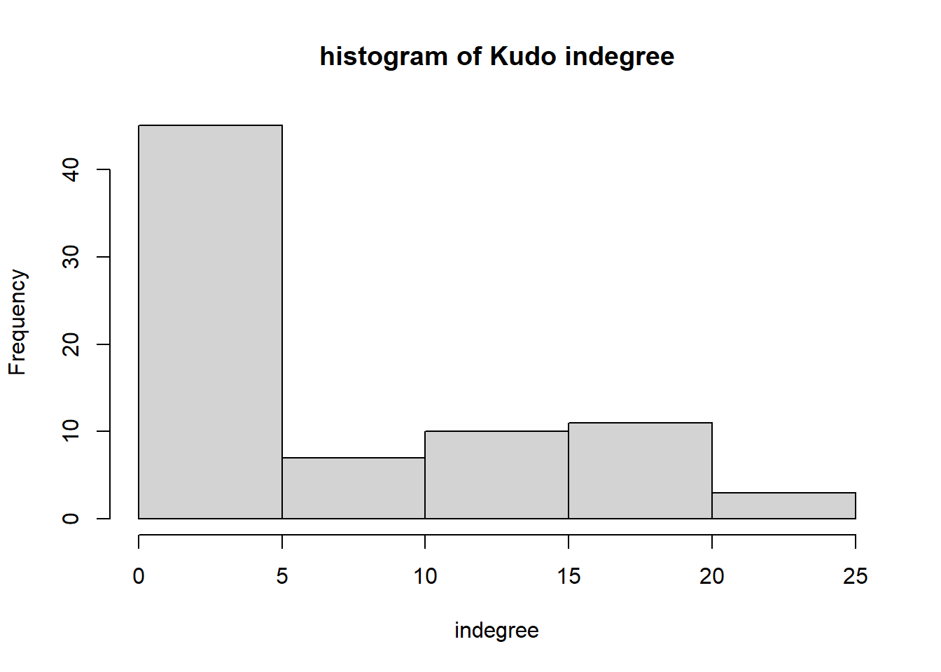

We can observe a Pareto-like-pattern: some give/receive most of the Kudos given, while most give/receive few.

2. Dyad-level

At the dyad-level: let’s see to what extent Kudos tend to be reciprocated between actors.

Club 1

# make igraph object for the club, at wave 1
df <- clubdata_rsiena_freq[[1]] # grab club 
knet <- df$depvars$kudonet # take Kudo network
knet1 <- knet[,,1] # take wave 1 only for now

# make an 'igraph object'
G1 <- igraph::graph_from_adjacency_matrix(knet1, mode = "directed", weighted = NULL, diag = TRUE, add.colnames = NA, add.rownames = NA)

# classify dyads
dyadcount <- igraph::dyad.census(G1)

# add the total number of dyads to the graph
dyadcount$total <- (vcount(G1)*(vcount(G1)-1))/2
dyadcount

#> $mut
#> [1] 30
#> 
#> $asym
#> [1] 5
#> 
#> $null
#> [1] 316
#> 
#> $total
#> [1] 351

# compare values with a random graph of the same size with the same density
dens <- igraph::graph.density(G1)
size <- igraph::vcount(G1)
trial <- 1000
recip <- rep(NA, trial)

for ( i in 1:trial ){
  random_graph <- igraph::erdos.renyi.game(n = size, p.or.m = dens, directed = TRUE)
  recip[i] <- igraph::dyad.census(random_graph)$mut
}

{hist(recip, main="number of reciprocated Kudos in random graph", xlab="", )
abline(v=dyadcount$mut, col="red", lwd=3)}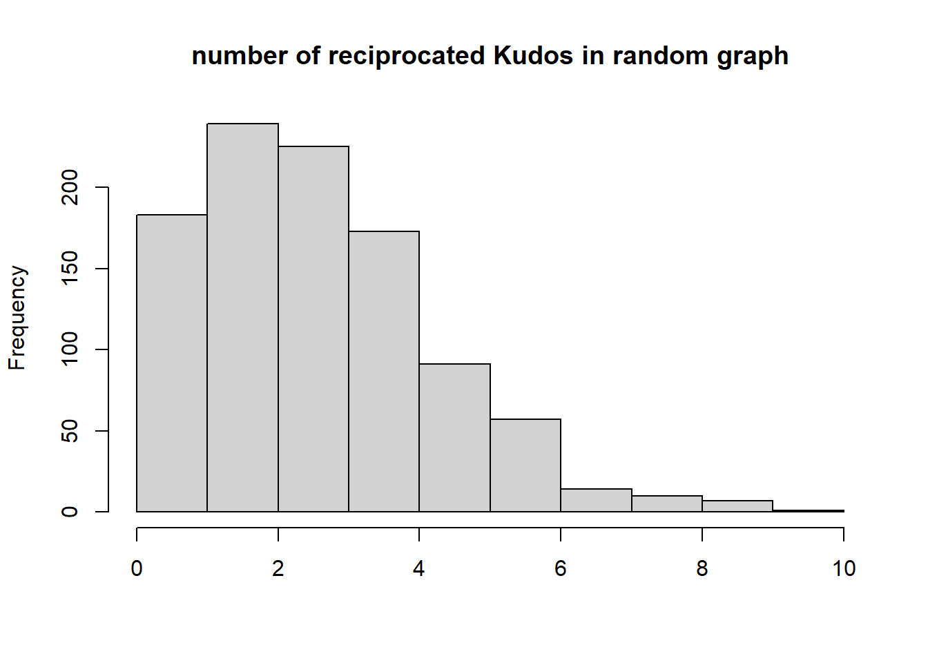

Club 2

# make igraph object for the club, at wave 1
df <- clubdata_rsiena_freq[[2]] # grab club 
knet <- df$depvars$kudonet # take Kudo network
knet1 <- knet[,,1] # take wave 1 only for now

# make an 'igraph object'
G1 <- igraph::graph_from_adjacency_matrix(knet1, mode = "directed", weighted = NULL, diag = TRUE, add.colnames = NA, add.rownames = NA)

# classify dyads
dyadcount <- igraph::dyad.census(G1)

# add the total number of dyads to the graph
dyadcount$total <- (vcount(G1)*(vcount(G1)-1))/2
dyadcount

#> $mut
#> [1] 231
#> 
#> $asym
#> [1] 99
#> 
#> $null
#> [1] 1323
#> 
#> $total
#> [1] 1653

# compare values with a random graph of the same size with the same density
dens <- igraph::graph.density(G1)
size <- igraph::vcount(G1)
trial <- 1000
recip <- rep(NA, trial)

for ( i in 1:trial ){
  random_graph <- igraph::erdos.renyi.game(n = size, p.or.m = dens, directed = TRUE)
  recip[i] <- igraph::dyad.census(random_graph)$mut
}

{hist(recip, main="number of reciprocated Kudos in random graph", xlab="", )
abline(v=dyadcount$mut, col="red", lwd=3)}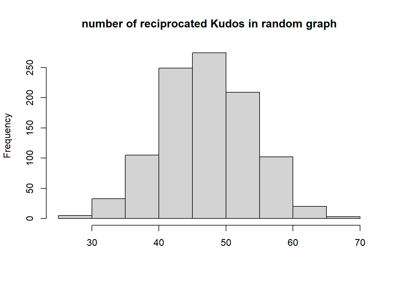

Club 3

# make igraph object for the club, at wave 1
df <- clubdata_rsiena_freq[[3]] # grab club 
knet <- df$depvars$kudonet # take Kudo network
knet1 <- knet[,,1] # take wave 1 only for now

# make an 'igraph object'
G1 <- igraph::graph_from_adjacency_matrix(knet1, mode = "directed", weighted = NULL, diag = TRUE, add.colnames = NA, add.rownames = NA)

# classify dyads
dyadcount <- igraph::dyad.census(G1)

# add the total number of dyads to the graph
dyadcount$total <- (vcount(G1)*(vcount(G1)-1))/2
dyadcount

#> $mut
#> [1] 91
#> 
#> $asym
#> [1] 104
#> 
#> $null
#> [1] 12366
#> 
#> $total
#> [1] 12561

# compare values with a random graph of the same size with the same density
dens <- igraph::graph.density(G1)
size <- igraph::vcount(G1)
trial <- 1000
recip <- rep(NA, trial)

for ( i in 1:trial ){
  random_graph <- igraph::erdos.renyi.game(n = size, p.or.m = dens, directed = TRUE)
  recip[i] <- igraph::dyad.census(random_graph)$mut
}

{hist(recip, main="number of reciprocated Kudos in random graph", xlab="", )
abline(v=dyadcount$mut, col="red", lwd=3)}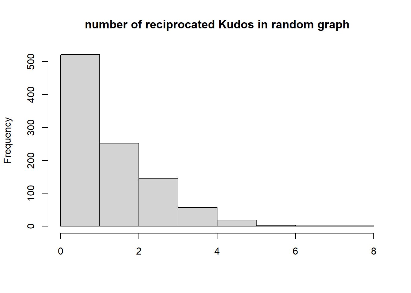

Club 4

# make igraph object for the club, at wave 1
df <- clubdata_rsiena_freq[[4]] # grab club 
knet <- df$depvars$kudonet # take Kudo network
knet1 <- knet[,,1] # take wave 1 only for now

# make an 'igraph object'
G1 <- igraph::graph_from_adjacency_matrix(knet1, mode = "directed", weighted = NULL, diag = TRUE, add.colnames = NA, add.rownames = NA)

# classify dyads
dyadcount <- igraph::dyad.census(G1)

# add the total number of dyads to the graph
dyadcount$total <- (vcount(G1)*(vcount(G1)-1))/2
dyadcount

#> $mut
#> [1] 7
#> 
#> $asym
#> [1] 2
#> 
#> $null
#> [1] 27
#> 
#> $total
#> [1] 36

# compare values with a random graph of the same size with the same density
dens <- igraph::graph.density(G1)
size <- igraph::vcount(G1)
trial <- 1000
recip <- rep(NA, trial)

for ( i in 1:trial ){
  random_graph <- igraph::erdos.renyi.game(n = size, p.or.m = dens, directed = TRUE)
  recip[i] <- igraph::dyad.census(random_graph)$mut
}

{hist(recip, main="number of reciprocated Kudos in random graph", xlab="", )
abline(v=dyadcount$mut, col="red", lwd=3)}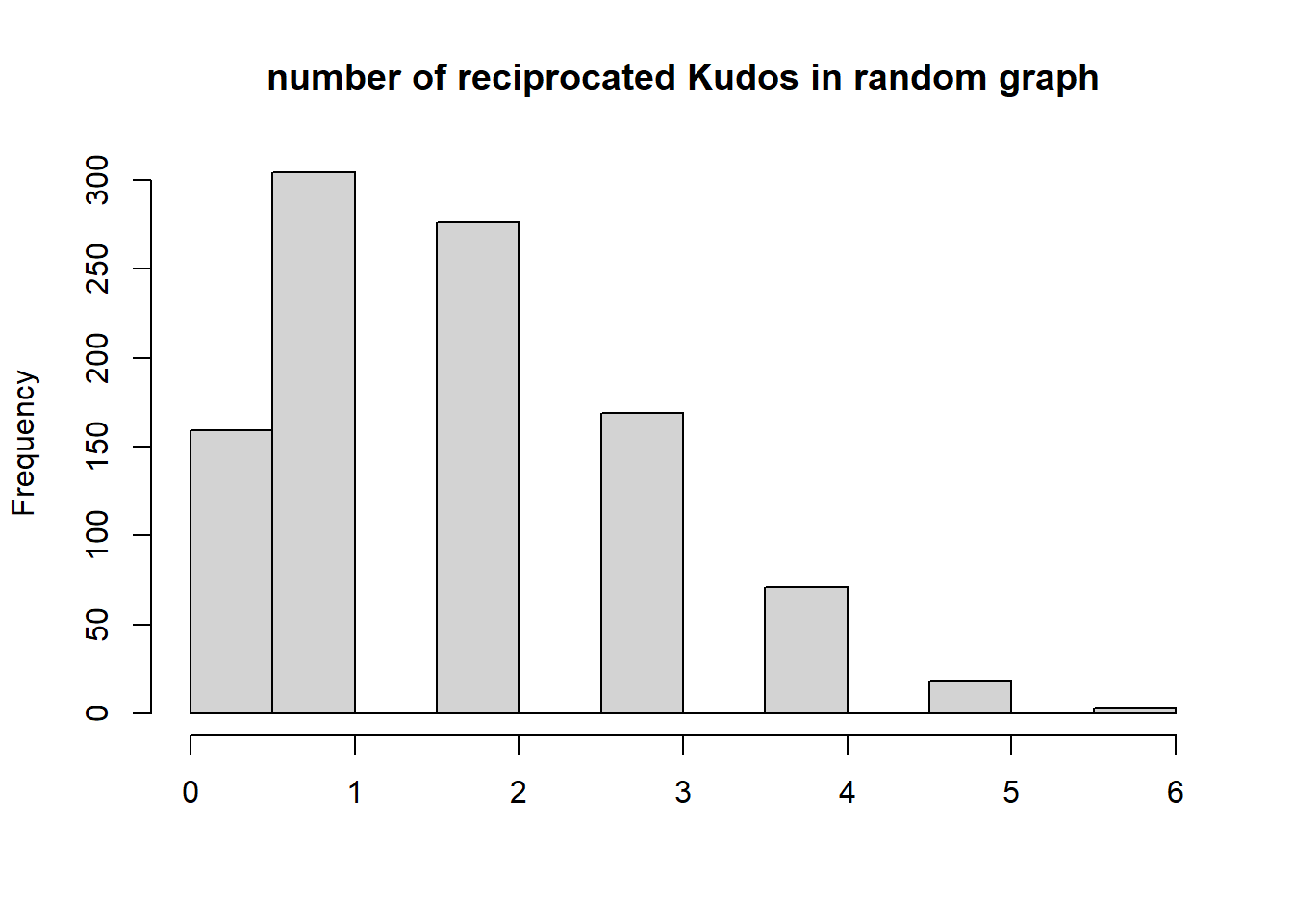

Club 5

# make igraph object for the club, at wave 1
df <- clubdata_rsiena_freq[[5]] # grab club 
knet <- df$depvars$kudonet # take Kudo network
knet1 <- knet[,,1] # take wave 1 only for now

# make an 'igraph object'
G1 <- igraph::graph_from_adjacency_matrix(knet1, mode = "directed", weighted = NULL, diag = TRUE, add.colnames = NA, add.rownames = NA)

# classify dyads
dyadcount <- igraph::dyad.census(G1)

# add the total number of dyads to the graph
dyadcount$total <- (vcount(G1)*(vcount(G1)-1))/2
dyadcount

#> $mut
#> [1] 195
#> 
#> $asym
#> [1] 119
#> 
#> $null
#> [1] 2536
#> 
#> $total
#> [1] 2850

# compare values with a random graph of the same size with the same density
dens <- igraph::graph.density(G1)
size <- igraph::vcount(G1)
trial <- 1000
recip <- rep(NA, trial)

for ( i in 1:trial ){
  random_graph <- igraph::erdos.renyi.game(n = size, p.or.m = dens, directed = TRUE)
  recip[i] <- igraph::dyad.census(random_graph)$mut
}

{hist(recip, main="number of reciprocated Kudos in random graph", xlab="", )
abline(v=dyadcount$mut, col="red", lwd=3)}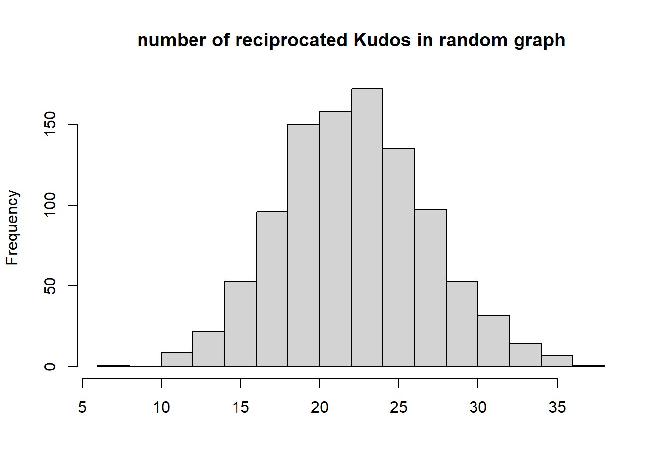

Conclusion: Kudos tend to be reciprocated!

---

Gender composition

Let’s investigate the gender composition of the club. We must retrieve gender from the object (note that we use the clubdata object, not the RSiena object). Then we make a categorical gender variable and plot it.

Club 1

df <- clubdata[[1]] # grab club 

# retrieve node-attribute gender from object
male <- df$male
female <- df$female
other <- df$other

# as factor
gender <- NA
gender <- ifelse(male == 1, "Male", gender)
gender <- ifelse(female == 1, "Female", gender)
gender <- ifelse(other == 1, "Other", gender)
gender <- ifelse(is.na(gender), "Missing", gender) # missing category

# make dataframe
df <- data.frame(
  gender = as.factor(c("Male", "Female", "Other", "Missing")),
  n = c(length(gender[gender == "Male"]), length(gender[gender == "Female"]), length(gender[gender == "Other"]), length(gender[gender == "Missing"])),
  freq = c(round((length(gender[gender=="Male"])/length(gender) *100), digits=1), round((length(gender[gender=="Female"])/length(gender) *100), digits=1), round((length(gender[gender=="Other"])/length(gender)*100), digits=1), round((length(gender[gender=="Missing"])/length(gender)*100), digits=1))
)

# plot
df %>%
  mutate(gender = fct_reorder(gender, -n)) %>%
           ggplot(aes(gender, n, fill=gender)) + 
           geom_bar(stat="identity", width=0.8) +
           geom_text(aes(label=paste0(freq,"%")), vjust=1.5, colour="white")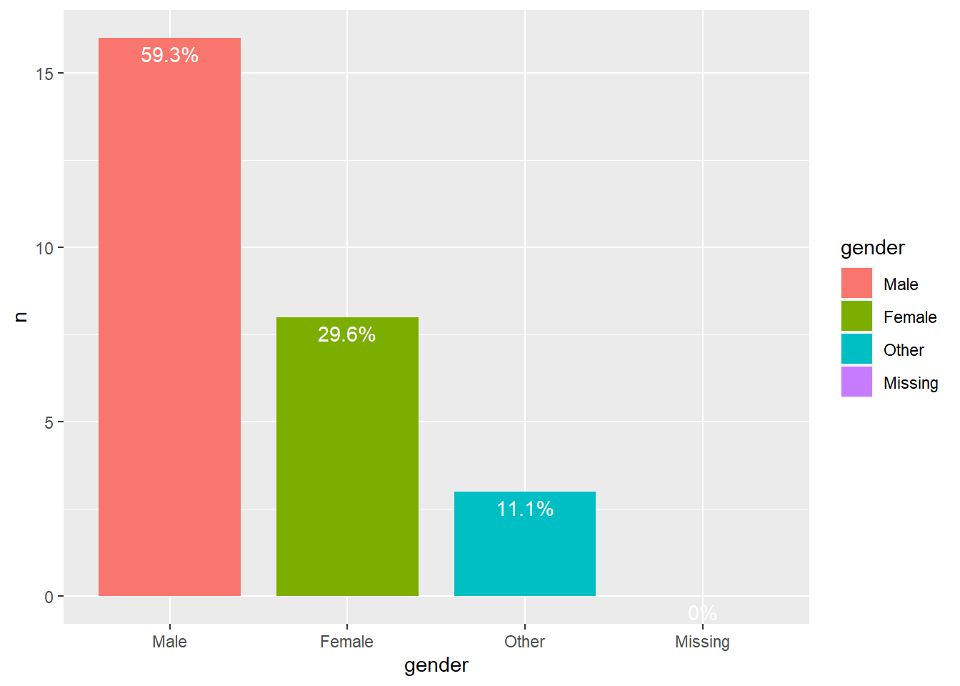

Club 2

df <- clubdata[[2]] # grab club 

# retrieve node-attribute gender from object
male <- df$male
female <- df$female
other <- df$other

# as factor
gender <- NA
gender <- ifelse(male == 1, "Male", gender)
gender <- ifelse(female == 1, "Female", gender)
gender <- ifelse(other == 1, "Other", gender)
gender <- ifelse(is.na(gender), "Missing", gender) # missing category

# make dataframe
df <- data.frame(
  gender = as.factor(c("Male", "Female", "Other", "Missing")),
  n = c(length(gender[gender == "Male"]), length(gender[gender == "Female"]), length(gender[gender == "Other"]), length(gender[gender == "Missing"])),
  freq = c(round((length(gender[gender=="Male"])/length(gender) *100), digits=1), round((length(gender[gender=="Female"])/length(gender) *100), digits=1), round((length(gender[gender=="Other"])/length(gender)*100), digits=1), round((length(gender[gender=="Missing"])/length(gender)*100), digits=1))
)

# plot
df %>%
  mutate(gender = fct_reorder(gender, -n)) %>%
           ggplot(aes(gender, n, fill=gender)) + 
           geom_bar(stat="identity", width=0.8) +
           geom_text(aes(label=paste0(freq,"%")), vjust=1.5, colour="white")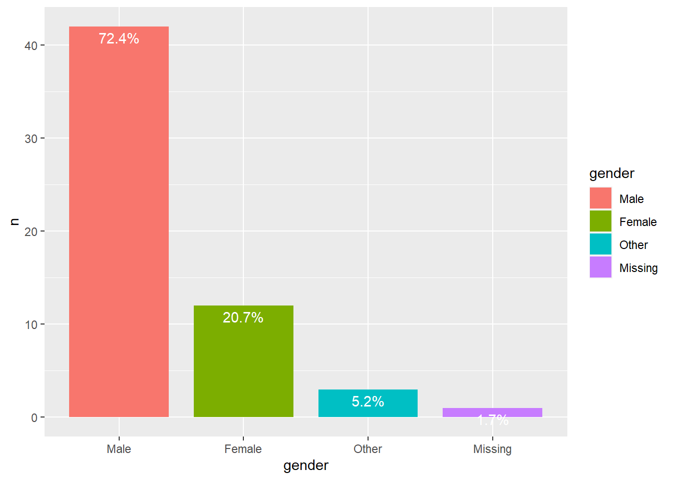

Club 3

df <- clubdata[[3]] # grab club 

# retrieve node-attribute gender from object
male <- df$male
female <- df$female
other <- df$other

# as factor
gender <- NA
gender <- ifelse(male == 1, "Male", gender)
gender <- ifelse(female == 1, "Female", gender)
gender <- ifelse(other == 1, "Other", gender)
gender <- ifelse(is.na(gender), "Missing", gender) # missing category

# make dataframe
df <- data.frame(
  gender = as.factor(c("Male", "Female", "Other", "Missing")),
  n = c(length(gender[gender == "Male"]), length(gender[gender == "Female"]), length(gender[gender == "Other"]), length(gender[gender == "Missing"])),
  freq = c(round((length(gender[gender=="Male"])/length(gender) *100), digits=1), round((length(gender[gender=="Female"])/length(gender) *100), digits=1), round((length(gender[gender=="Other"])/length(gender)*100), digits=1), round((length(gender[gender=="Missing"])/length(gender)*100), digits=1))
)

# plot
df %>%
  mutate(gender = fct_reorder(gender, -n)) %>%
           ggplot(aes(gender, n, fill=gender)) + 
           geom_bar(stat="identity", width=0.8) +
           geom_text(aes(label=paste0(freq,"%")), vjust=1.5, colour="white")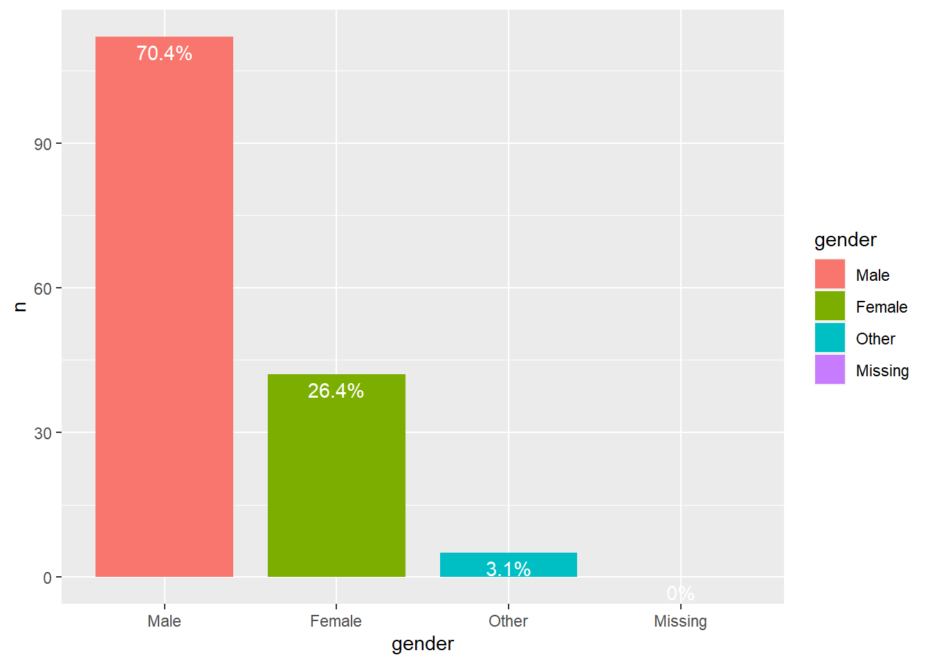

Club 4

df <- clubdata[[4]] # grab club 

# retrieve node-attribute gender from object
male <- df$male
female <- df$female
other <- df$other

# as factor
gender <- NA
gender <- ifelse(male == 1, "Male", gender)
gender <- ifelse(female == 1, "Female", gender)
gender <- ifelse(other == 1, "Other", gender)
gender <- ifelse(is.na(gender), "Missing", gender) # missing category

# make dataframe
df <- data.frame(
  gender = as.factor(c("Male", "Female", "Other", "Missing")),
  n = c(length(gender[gender == "Male"]), length(gender[gender == "Female"]), length(gender[gender == "Other"]), length(gender[gender == "Missing"])),
  freq = c(round((length(gender[gender=="Male"])/length(gender) *100), digits=1), round((length(gender[gender=="Female"])/length(gender) *100), digits=1), round((length(gender[gender=="Other"])/length(gender)*100), digits=1), round((length(gender[gender=="Missing"])/length(gender)*100), digits=1))
)

# plot
df %>%
  mutate(gender = fct_reorder(gender, -n)) %>%
           ggplot(aes(gender, n, fill=gender)) + 
           geom_bar(stat="identity", width=0.8) +
           geom_text(aes(label=paste0(freq,"%")), vjust=1.5, colour="white")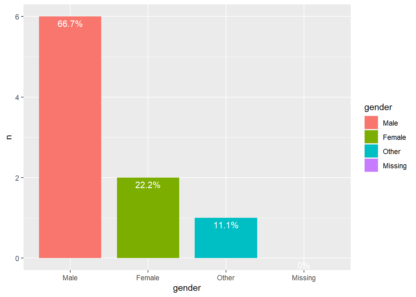

Club 5

df <- clubdata[[5]] # grab club 

# retrieve node-attribute gender from object
male <- df$male
female <- df$female
other <- df$other

# as factor
gender <- NA
gender <- ifelse(male == 1, "Male", gender)
gender <- ifelse(female == 1, "Female", gender)
gender <- ifelse(other == 1, "Other", gender)
gender <- ifelse(is.na(gender), "Missing", gender) # missing category

# make dataframe
df <- data.frame(
  gender = as.factor(c("Male", "Female", "Other", "Missing")),
  n = c(length(gender[gender == "Male"]), length(gender[gender == "Female"]), length(gender[gender == "Other"]), length(gender[gender == "Missing"])),
  freq = c(round((length(gender[gender=="Male"])/length(gender) *100), digits=1), round((length(gender[gender=="Female"])/length(gender) *100), digits=1), round((length(gender[gender=="Other"])/length(gender)*100), digits=1), round((length(gender[gender=="Missing"])/length(gender)*100), digits=1))
)

# plot
df %>%
  mutate(gender = fct_reorder(gender, -n)) %>%
           ggplot(aes(gender, n, fill=gender)) + 
           geom_bar(stat="identity", width=0.8) +
           geom_text(aes(label=paste0(freq,"%")), vjust=1.5, colour="white")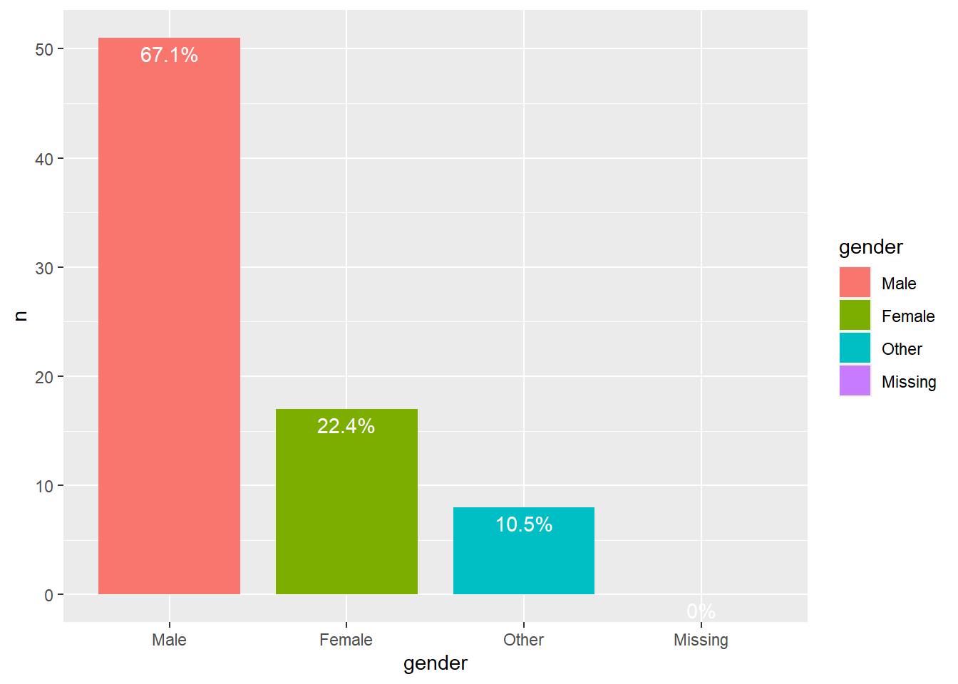

We can see that in all clubs men are the majority.

---

Gender segregation

Let’s now investigate segregation along gender in the kudos network.

Let’s start with describing the total density and intra- (same gender) and intergroup (different gender) densities. We also calculate the Coleman Homophily index for gender, which reflects gender segregation while taking into account the relative group size of gender categories.

Club 1

df <- clubdata_rsiena_freq[[1]] # grab club 
df2 <- clubdata[[1]]

knet <- df$depvars$kudonet # take Kudo network
knet1 <- knet[,,1] # take wave 1 only for now

# for some reason constructing the dyad-similarity matrix for gender with the rsiena object did not work, so we use the clubdata.RData.
male <- df2$male
female <- df2$female
other <- df2$other

gender <- NA
gender <- ifelse(male == 1, "Male", gender)
gender <- ifelse(female == 1, "Female", gender)
gender <- ifelse(other == 1, "Other", gender)
gender <- ifelse(is.na(gender), "Missing", gender) # missing category

# construct dyad similarity matrix
gender_m <- fhomomat(gender)


# make object to store results
desmat <- matrix(NA, nrow=4, ncol=1)

# use functions
desmat[1, 1] <- fdensity(knet1)
desmat[2, 1] <- fdensityintra(knet1, gender_m)
desmat[3, 1] <- fdensityinter(knet1, gender_m)
desmat[4, 1] <- fscolnet(knet1, gender)

colnames(desmat) <- c("Kudos network")
rownames(desmat) <- c("total density", "same gender density", "different gender density", "Coleman's homophily index")



knitr::kable(desmat, digits=3, "html", caption="Gender segregation in friendship and kudo network") %>% 
  kableExtra::kable_styling(bootstrap_options = c("striped", "hover"))

Gender segregation in friendship and kudo network

	Kudos network
total density	0.118
same gender density	0.151
different gender density	0.086
Coleman’s homophily index	0.232

Club 2

df <- clubdata_rsiena_freq[[2]] # grab club 
df2 <- clubdata[[2]]

knet <- df$depvars$kudonet # take Kudo network
knet1 <- knet[,,1] # take wave 1 only for now

# for some reason constructing the dyad-similarity matrix for gender with the rsiena object did not work, so we use the clubdata.RData.
male <- df2$male
female <- df2$female
other <- df2$other

gender <- NA
gender <- ifelse(male == 1, "Male", gender)
gender <- ifelse(female == 1, "Female", gender)
gender <- ifelse(other == 1, "Other", gender)
gender <- ifelse(is.na(gender), "Missing", gender) # missing category

# construct dyad similarity matrix
gender_m <- fhomomat(gender)


# make object to store results
desmat <- matrix(NA, nrow=4, ncol=1)

# use functions
desmat[1, 1] <- fdensity(knet1)
desmat[2, 1] <- fdensityintra(knet1, gender_m)
desmat[3, 1] <- fdensityinter(knet1, gender_m)
desmat[4, 1] <- fscolnet(knet1, gender)

colnames(desmat) <- c("Kudos network")
rownames(desmat) <- c("total density", "same gender density", "different gender density", "Coleman's homophily index")



knitr::kable(desmat, digits=3, "html", caption="Gender segregation in friendship and kudo network") %>% 
  kableExtra::kable_styling(bootstrap_options = c("striped", "hover"))

Gender segregation in friendship and kudo network

	Kudos network
total density	0.189
same gender density	0.250
different gender density	0.103
Coleman’s homophily index	0.343

Club 3

df <- clubdata_rsiena_freq[[3]] # grab club 
df2 <- clubdata[[3]]

knet <- df$depvars$kudonet # take Kudo network
knet1 <- knet[,,1] # take wave 1 only for now

# for some reason constructing the dyad-similarity matrix for gender with the rsiena object did not work, so we use the clubdata.RData.
male <- df2$male
female <- df2$female
other <- df2$other

gender <- NA
gender <- ifelse(male == 1, "Male", gender)
gender <- ifelse(female == 1, "Female", gender)
gender <- ifelse(other == 1, "Other", gender)
gender <- ifelse(is.na(gender), "Missing", gender) # missing category

# construct dyad similarity matrix
gender_m <- fhomomat(gender)


# make object to store results
desmat <- matrix(NA, nrow=4, ncol=1)

# use functions
desmat[1, 1] <- fdensity(knet1)
desmat[2, 1] <- fdensityintra(knet1, gender_m)
desmat[3, 1] <- fdensityinter(knet1, gender_m)
desmat[4, 1] <- fscolnet(knet1, gender)

colnames(desmat) <- c("Kudos network")
rownames(desmat) <- c("total density", "same gender density", "different gender density", "Coleman's homophily index")



knitr::kable(desmat, digits=3, "html", caption="Gender segregation in friendship and kudo network") %>% 
  kableExtra::kable_styling(bootstrap_options = c("striped", "hover"))

Gender segregation in friendship and kudo network

	Kudos network
total density	0.017
same gender density	0.017
different gender density	0.018
Coleman’s homophily index	0.040

Club 4

df <- clubdata_rsiena_freq[[4]] # grab club 
df2 <- clubdata[[4]]

knet <- df$depvars$kudonet # take Kudo network
knet1 <- knet[,,1] # take wave 1 only for now

# for some reason constructing the dyad-similarity matrix for gender with the rsiena object did not work, so we use the clubdata.RData.
male <- df2$male
female <- df2$female
other <- df2$other

gender <- NA
gender <- ifelse(male == 1, "Male", gender)
gender <- ifelse(female == 1, "Female", gender)
gender <- ifelse(other == 1, "Other", gender)
gender <- ifelse(is.na(gender), "Missing", gender) # missing category

# construct dyad similarity matrix
gender_m <- fhomomat(gender)


# make object to store results
desmat <- matrix(NA, nrow=4, ncol=1)

# use functions
desmat[1, 1] <- fdensity(knet1)
desmat[2, 1] <- fdensityintra(knet1, gender_m)
desmat[3, 1] <- fdensityinter(knet1, gender_m)
desmat[4, 1] <- fscolnet(knet1, gender)

colnames(desmat) <- c("Kudos network")
rownames(desmat) <- c("total density", "same gender density", "different gender density", "Coleman's homophily index")



knitr::kable(desmat, digits=3, "html", caption="Gender segregation in friendship and kudo network") %>% 
  kableExtra::kable_styling(bootstrap_options = c("striped", "hover"))

Gender segregation in friendship and kudo network

	Kudos network
total density	0.381
same gender density	0.286
different gender density	0.429
Coleman’s homophily index	-0.347

Club 5

df <- clubdata_rsiena_freq[[5]] # grab club 
df2 <- clubdata[[5]]

knet <- df$depvars$kudonet # take Kudo network
knet1 <- knet[,,1] # take wave 1 only for now

# for some reason constructing the dyad-similarity matrix for gender with the rsiena object did not work, so we use the clubdata.RData.
male <- df2$male
female <- df2$female
other <- df2$other

gender <- NA
gender <- ifelse(male == 1, "Male", gender)
gender <- ifelse(female == 1, "Female", gender)
gender <- ifelse(other == 1, "Other", gender)
gender <- ifelse(is.na(gender), "Missing", gender) # missing category

# construct dyad similarity matrix
gender_m <- fhomomat(gender)


# make object to store results
desmat <- matrix(NA, nrow=4, ncol=1)

# use functions
desmat[1, 1] <- fdensity(knet1)
desmat[2, 1] <- fdensityintra(knet1, gender_m)
desmat[3, 1] <- fdensityinter(knet1, gender_m)
desmat[4, 1] <- fscolnet(knet1, gender)

colnames(desmat) <- c("Kudos network")
rownames(desmat) <- c("total density", "same gender density", "different gender density", "Coleman's homophily index")



knitr::kable(desmat, digits=3, "html", caption="Gender segregation in friendship and kudo network") %>% 
  kableExtra::kable_styling(bootstrap_options = c("striped", "hover"))

Gender segregation in friendship and kudo network

	Kudos network
total density	0.122
same gender density	0.117
different gender density	0.129
Coleman’s homophily index	0.025

Density in the kudos network is not much higher within-gender than between-genders, though this ratio differs per club (and in one clubs between-gender kudos are more common).

Coleman’s Homophily indices vary across clubs. In some clubs there is slight gender segregation (or same-gender preference) in kudos ties (values higher than 0, but rather close to 0), though in others members tend to give kudos to others outside their own gender group (values lower than 0).

---

Behavior

We plotted the development of the mean of running attributes (Figure 3 of the manuscript). The script to replicate this plot can be found here.

---

Correlation between frequency and volume

Let’s plot the relation between frequency in times per week and volume in hours per week. We also calculate Kendall’s tau-b, i.e. a non-parametric measure of correlation on ranks (cf. Khamis (2008)).

Club 1

df <- clubdata[[1]] # grab club 
df <- data.frame(x = as.matrix(df$time_run), y = as.matrix(df$freq_run))

c <- cor.test(df$x, df$y, method="kendall")

plot(df, type="b", 
     main = "Relation between weekly running variables: frequency and (half) hours",
     sub = "Note: running frequency capped with a maximum of 7, hours with a maximum of 7",
     xlab = "Hours per week", ylab = "sessions per week",
     col="blue", lwd=c(1,rep(6,10000))) + 
  text(x = 1.7, y = 5, round(c$estimate, digits=2)) +
  text(x = .7, y = 5, "Kendall's tau-b =")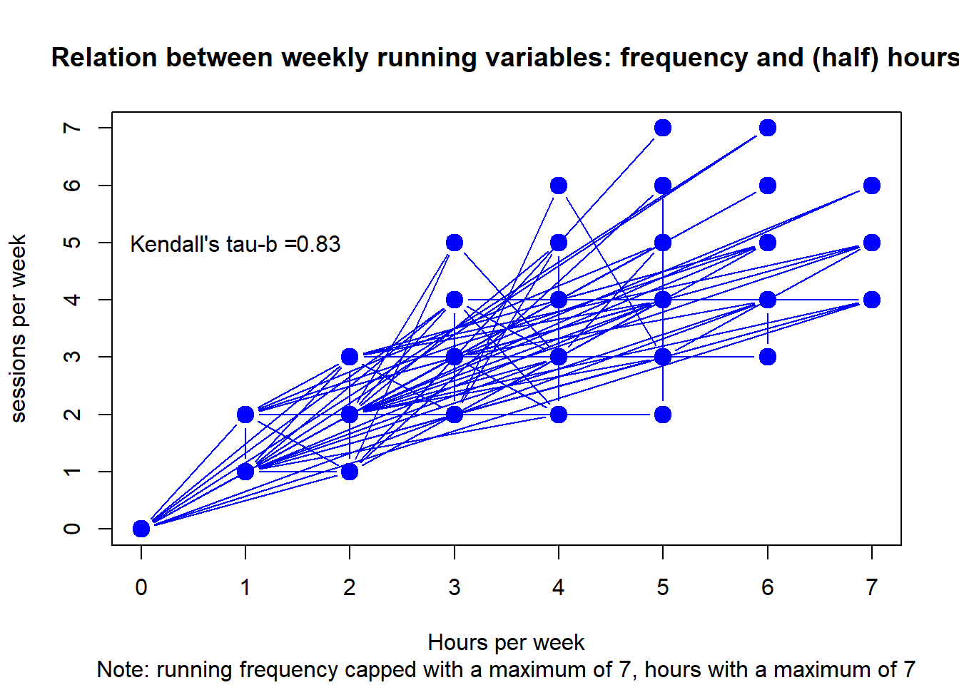

#> integer(0)

Club 2

df <- clubdata[[2]] # grab club 
df <- data.frame(x = as.matrix(df$time_run), y = as.matrix(df$freq_run))
c <- cor.test(df$x,df$y,method="kendall")

plot(df, type="b", 
     main = "Relation between weekly running variables: frequency and hours",
     sub = "Note: running frequency capped with a maximum of 7, hours with a maximum of 7",
     xlab = "hours per week", ylab = "sessions per week",
     col="blue", lwd=c(1,rep(6,10000))) + 
  text(x = 1.7, y = 5, round(c$estimate, digits=2)) +
  text(x = .7, y = 5, "Kendall's tau-b =")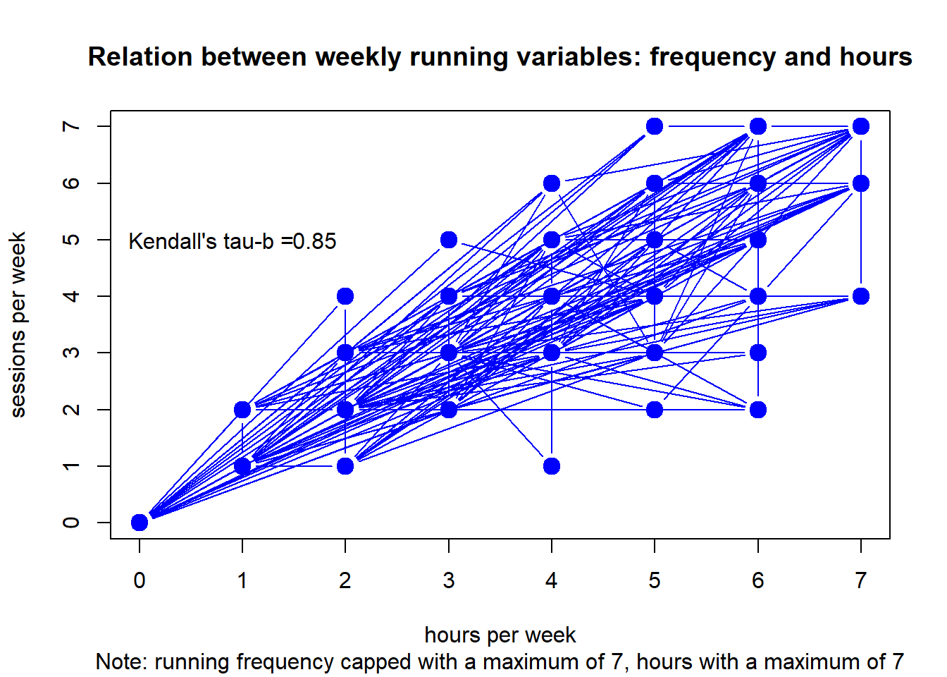

#> integer(0)

Club 3

df <- clubdata[[3]] # grab club 
df <- data.frame(x = as.matrix(df$time_run), y = as.matrix(df$freq_run))
c <- cor.test(df$x,df$y,method="kendall")

plot(df, type="b", 
     main = "Relation between weekly running variables: frequency and hours",
     sub = "Note: running frequency capped with a maximum of 7, hours with a maximum of 7",
     xlab = "hours per week", ylab = "sessions per week",
     col="blue", lwd=c(1,rep(6,10000))) + 
  text(x = 1.7, y = 5, round(c$estimate, digits=2)) +
  text(x = .7, y = 5, "Kendall's tau-b =")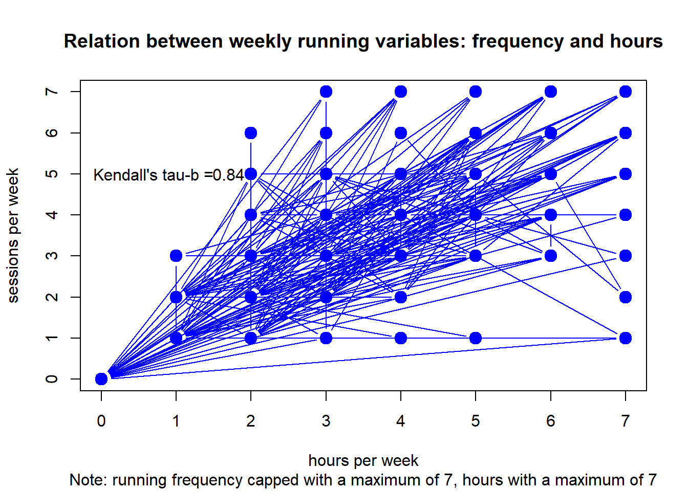

#> integer(0)

Club 4

df <- clubdata[[4]] # grab club 
df <- data.frame(x = as.matrix(df$time_run), y = as.matrix(df$freq_run))
c <- cor.test(df$x,df$y,method="kendall")

plot(df, type="b", 
     main = "Relation between weekly running variables: frequency and hours",
     sub = "Note: running frequency capped with a maximum of 7, hours with a maximum of 7",
     xlab = "hours per week", ylab = "sessions per week",
     col="blue", lwd=c(1,rep(6,10000))) + 
  text(x = 1.5, y = 5, round(c$estimate, digits=2)) +
  text(x = .7, y = 5, "Kendall's tau-b =")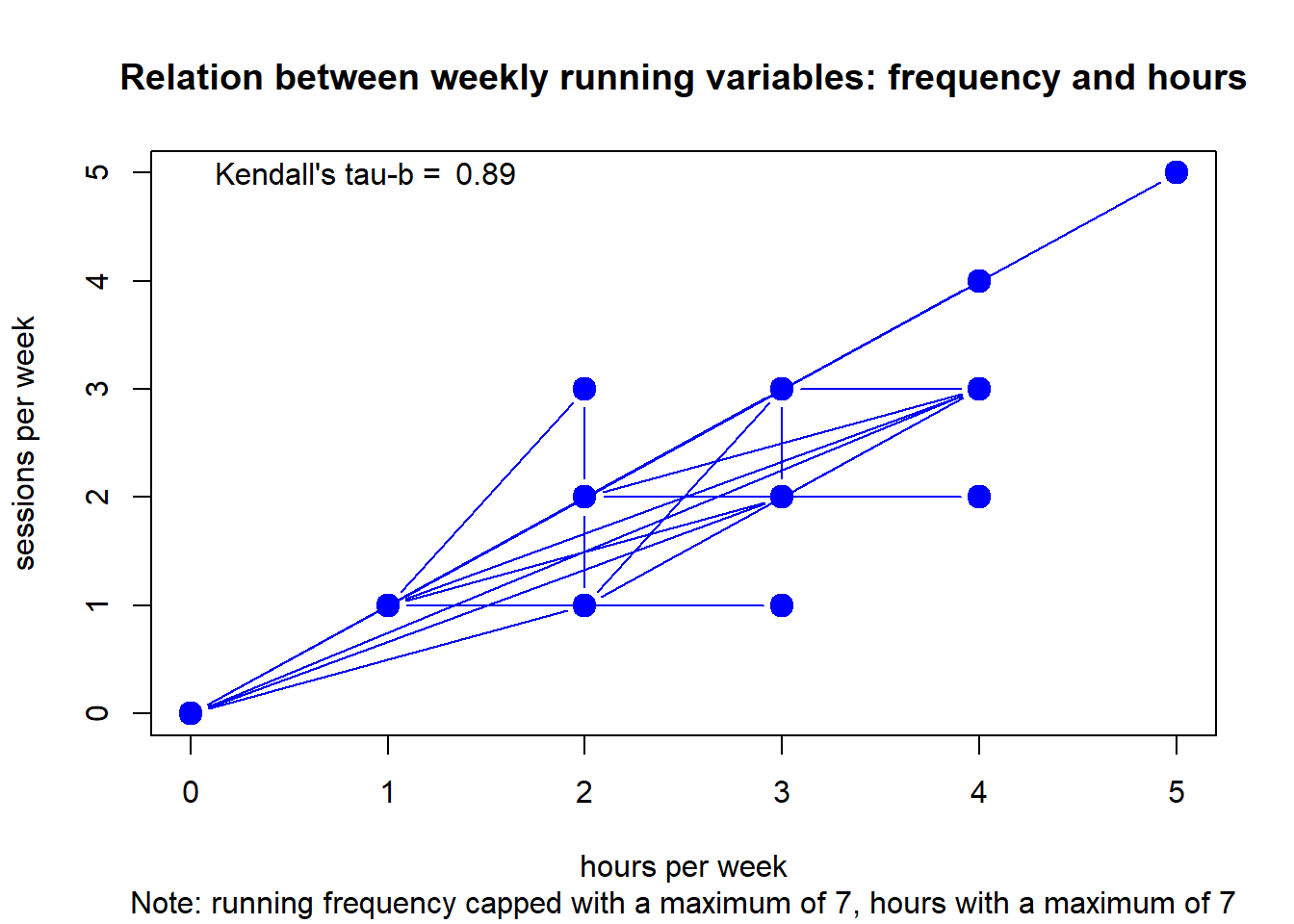

#> integer(0)

Club 5

df <- clubdata[[5]] # grab club 
df <- data.frame(x = as.matrix(df$time_run), y = as.matrix(df$freq_run))
c <- cor.test(df$x,df$y,method="kendall")

plot(df, type="b", 
     main = "Relation between weekly running variables: frequency and hours",
     sub = "Note: running frequency capped with a maximum of 7, hours with a maximum of 7",
     xlab = "hours per week", ylab = "sessions per week",
     col="blue", lwd=c(1,rep(6,10000))) + 
  text(x = 2, y = 7, round(c$estimate, digits=2)) +
  text(x = .7, y = 7, "Kendall's tau-b =")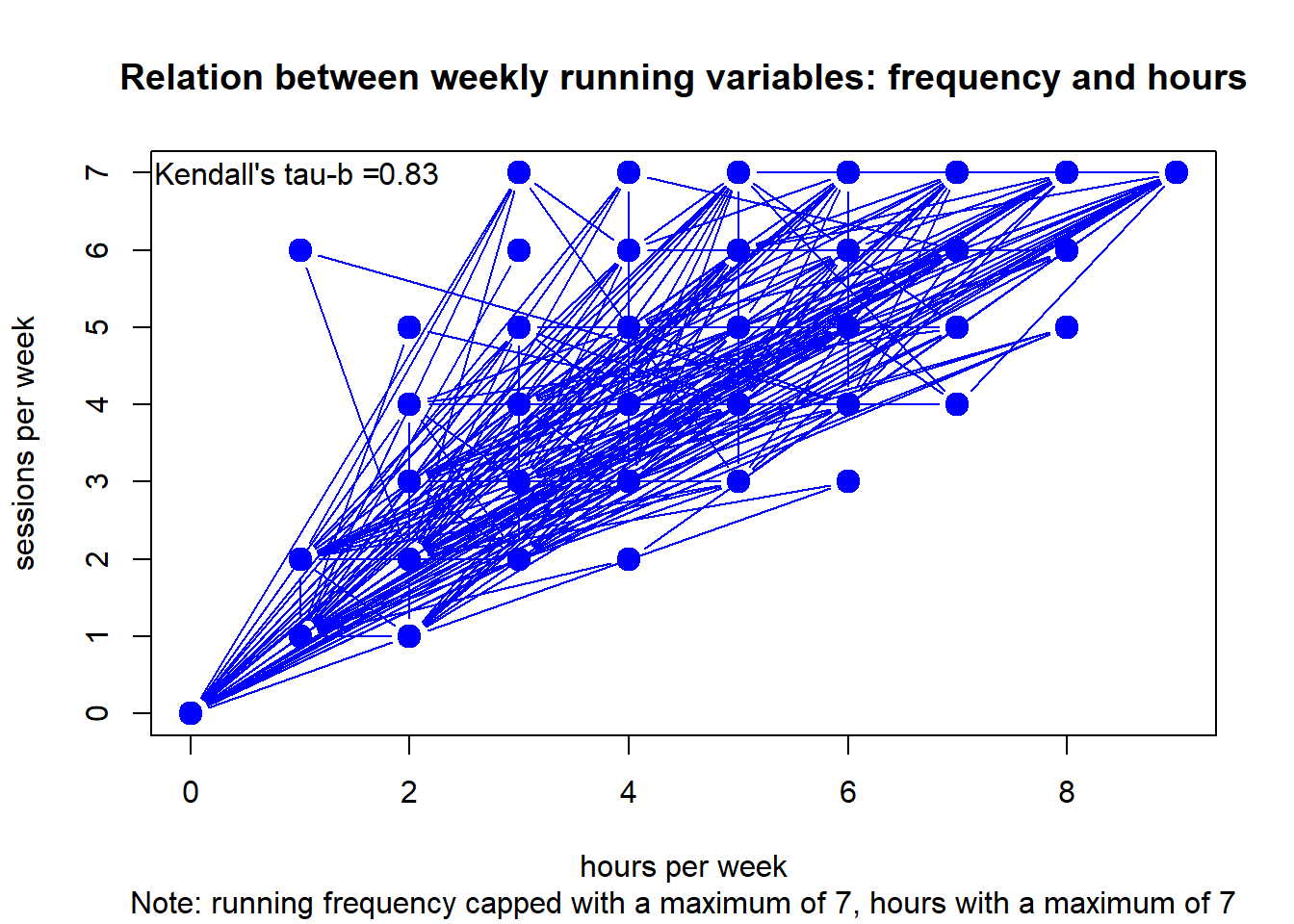

#> integer(0)

Although frequency and duration are strongly related, there is some invariance.

---

Network autocorrelation

We have now covered the sport activity levels of our club-athletes, and the extent to which kudos-associations are segregated along gender. Last, we will explore if kudos-ties are also segregated along activity levels. Or in other words: do people with similar activity levels tend to socialize to a greater extent - by exchanging kudos - even when taking into account the opportunity structures for ‘interacting’ with (dis)similar others?

We use Moran’s I spatial autocorrelation measure for this, which is the correlation between the behavioral score of actor i and the (total/mean) behavioral score of alters j to whom i is connected directly. We also calculated Moran’s I by including the behavioral scores of the actors h to whom i is indirectly tied, and used the negative exponential function as described by Chen (2013) as a distance-decay function for assigning weights.

Club 1

df <- clubdata[[1]] # grab club 

# get behavioral data
# at time t=1
t=1
freq1 <- df$freq_run[,,t] # running frequencies wave 1
vol1 <- df$time_run[,,t] # running volume wave 1

# exclude NAs 
na <- which(is.na(freq1))
freq1 <- freq1[-na]
vol1 <- vol1[-na]

# get kudos net
knet1 <- df$kudo[,,t]
# exclude NAs
knet1 <- knet1[-na,-na]

# as network object
knet1 <- network::as.network(knet1)

# we include geodistances: shortest path lengths from i to j
geodistances <- sna::geodist(knet1, count.paths=T)
geodistances <- geodistances$gdist 

# set the distance 'to yourself' to 'Inf'
diag(geodistances) <- Inf

# first calculate Moran's i for alters at distance 1.
weights1 <- geodistances == 1

# and use the negative exponential distance-decay function
weights2 <- exp(-geodistances)

# calculate Moran's I
# for distance-1 and with distance decay, in the kudos network, for frequency and volume  respectively
# we do not row standardize!
Mfreq <- fMoran.I(freq1, scaled = FALSE, weight = weights1, na.rm = TRUE, rowstandardize = FALSE)
Mfreq_distd <- fMoran.I(freq1, scaled = FALSE, weight = weights2, na.rm = TRUE, rowstandardize = FALSE)

Mvol <- fMoran.I(vol1, scaled = FALSE, weight = weights1, na.rm = TRUE, rowstandardize = FALSE)
Mvol_distd <- fMoran.I(vol1, scaled = FALSE, weight = weights2, na.rm = TRUE, rowstandardize = FALSE)

# make object to store results
# 1. frequency
f_mat <- matrix(NA, nrow=2, ncol=4)

f_mat[1,1] <- Mfreq$observed
f_mat[1,2] <- Mfreq$expected
f_mat[1,3] <- Mfreq$sd
f_mat[1,4] <- Mfreq$p.value
f_mat[2,1] <- Mfreq_distd$observed
f_mat[2,2] <- Mfreq_distd$expected
f_mat[2,3] <- Mfreq_distd$sd
f_mat[2,4] <- Mfreq_distd$p.value

# 2. volume
v_mat <- matrix(NA, nrow=2, ncol=4)
v_mat[1,1] <- Mvol$observed
v_mat[1,2] <- Mvol$expected
v_mat[1,3] <- Mvol$sd
v_mat[1,4] <- Mvol$p.value
v_mat[2,1] <- Mvol_distd$observed
v_mat[2,2] <- Mvol_distd$expected
v_mat[2,3] <- Mvol_distd$sd
v_mat[2,4] <- Mvol_distd$p.value

colnames(f_mat) <- colnames(v_mat) <- c("observed", "expected", "sd", "p-value")
rownames(f_mat) <- rownames(v_mat) <- c("direct kudos ties", "direct and indirect kudos ties (distance-decay)")

knitr::kable(f_mat, digits=2, "html", caption="Moran's I statistic for spatial autocorrelation based on geodistances and weekly running frequency") %>% 
  kableExtra::kable_styling(bootstrap_options = c("striped", "hover"))

Moran’s I statistic for spatial autocorrelation based on geodistances and weekly running frequency

	observed	expected	sd	p-value
direct kudos ties	0.01	-0.04	0.13	0.66
direct and indirect kudos ties (distance-decay)	0.00	-0.04	0.08	0.57

knitr::kable(v_mat, digits=2, "html", caption="Moran's I statistic for spatial autocorrelation based on geodistances and monthly running volume") %>% 
  kableExtra::kable_styling(bootstrap_options = c("striped", "hover"))

Moran’s I statistic for spatial autocorrelation based on geodistances and monthly running volume

	observed	expected	sd	p-value
direct kudos ties	-0.01	-0.04	0.13	0.80
direct and indirect kudos ties (distance-decay)	-0.01	-0.04	0.08	0.71

Club 2

df <- clubdata[[2]] # grab club 

# get behavioral data
# at time t=1
t=1
freq1 <- df$freq_run[,,t] # running frequencies wave 1
vol1 <- df$time_run[,,t] # running volume wave 1

# exclude NAs 
na <- which(is.na(freq1))
freq1 <- freq1[-na]
vol1 <- vol1[-na]

# get kudos net
knet1 <- df$kudo[,,t]
# exclude NAs
knet1 <- knet1[-na,-na]

# as network object
knet1 <- network::as.network(knet1)

# we include geodistances: shortest path lengths from i to j
geodistances <- sna::geodist(knet1, count.paths=T)
geodistances <- geodistances$gdist 

# set the distance 'to yourself' to 'Inf'
diag(geodistances) <- Inf

# first calculate Moran's i for alters at distance 1.
weights1 <- geodistances == 1

# and use the negative exponential distance-decay function
weights2 <- exp(-geodistances)

# calculate Moran's I
# for distance-1 and with distance decay, in the kudos network, for frequency and volume  respectively
# we do not row standardize!
Mfreq <- fMoran.I(freq1, scaled = FALSE, weight = weights1, na.rm = TRUE, rowstandardize = FALSE)
Mfreq_distd <- fMoran.I(freq1, scaled = FALSE, weight = weights2, na.rm = TRUE, rowstandardize = FALSE)

Mvol <- fMoran.I(vol1, scaled = FALSE, weight = weights1, na.rm = TRUE, rowstandardize = FALSE)
Mvol_distd <- fMoran.I(vol1, scaled = FALSE, weight = weights2, na.rm = TRUE, rowstandardize = FALSE)

# make object to store results
# 1. frequency
f_mat <- matrix(NA, nrow=2, ncol=4)

f_mat[1,1] <- Mfreq$observed
f_mat[1,2] <- Mfreq$expected
f_mat[1,3] <- Mfreq$sd
f_mat[1,4] <- Mfreq$p.value
f_mat[2,1] <- Mfreq_distd$observed
f_mat[2,2] <- Mfreq_distd$expected
f_mat[2,3] <- Mfreq_distd$sd
f_mat[2,4] <- Mfreq_distd$p.value

# 2. volume
v_mat <- matrix(NA, nrow=2, ncol=4)
v_mat[1,1] <- Mvol$observed
v_mat[1,2] <- Mvol$expected
v_mat[1,3] <- Mvol$sd
v_mat[1,4] <- Mvol$p.value
v_mat[2,1] <- Mvol_distd$observed
v_mat[2,2] <- Mvol_distd$expected
v_mat[2,3] <- Mvol_distd$sd
v_mat[2,4] <- Mvol_distd$p.value

colnames(f_mat) <- colnames(v_mat) <- c("observed", "expected", "sd", "p-value")
rownames(f_mat) <- rownames(v_mat) <- c("direct kudos ties", "direct and indirect kudos ties (distance-decay)")

knitr::kable(f_mat, digits=2, "html", caption="Moran's I statistic for spatial autocorrelation based on geodistances and weekly running frequency") %>% 
  kableExtra::kable_styling(bootstrap_options = c("striped", "hover"))

Moran’s I statistic for spatial autocorrelation based on geodistances and weekly running frequency

	observed	expected	sd	p-value
direct kudos ties	0.17	-0.02	0.04	0
direct and indirect kudos ties (distance-decay)	0.05	-0.02	0.01	0

knitr::kable(v_mat, digits=2, "html", caption="Moran's I statistic for spatial autocorrelation based on geodistances and monthly running volume") %>% 
  kableExtra::kable_styling(bootstrap_options = c("striped", "hover"))

Moran’s I statistic for spatial autocorrelation based on geodistances and monthly running volume

	observed	expected	sd	p-value
direct kudos ties	0.21	-0.02	0.04	0
direct and indirect kudos ties (distance-decay)	0.06	-0.02	0.01	0

Club 3

df <- clubdata[[3]] # grab club 

# get behavioral data
# at time t=1
t=1
freq1 <- df$freq_run[,,t] # running frequencies wave 1
vol1 <- df$time_run[,,t] # running volume wave 1

# exclude NAs 
na <- which(is.na(freq1))
freq1 <- freq1[-na]
vol1 <- vol1[-na]

# get kudos net
knet1 <- df$kudo[,,t]
# exclude NAs
knet1 <- knet1[-na,-na]

# as network object
knet1 <- network::as.network(knet1)

# we include geodistances: shortest path lengths from i to j
geodistances <- sna::geodist(knet1, count.paths=T)
geodistances <- geodistances$gdist 

# set the distance 'to yourself' to 'Inf'
diag(geodistances) <- Inf

# first calculate Moran's i for alters at distance 1.
weights1 <- geodistances == 1

# and use the negative exponential distance-decay function
weights2 <- exp(-geodistances)

# calculate Moran's I
# for distance-1 and with distance decay, in the kudos network, for frequency and volume  respectively
# we do not row standardize!
Mfreq <- fMoran.I(freq1, scaled = FALSE, weight = weights1, na.rm = TRUE, rowstandardize = FALSE)
Mfreq_distd <- fMoran.I(freq1, scaled = FALSE, weight = weights2, na.rm = TRUE, rowstandardize = FALSE)

Mvol <- fMoran.I(vol1, scaled = FALSE, weight = weights1, na.rm = TRUE, rowstandardize = FALSE)
Mvol_distd <- fMoran.I(vol1, scaled = FALSE, weight = weights2, na.rm = TRUE, rowstandardize = FALSE)

# make object to store results
# 1. frequency
f_mat <- matrix(NA, nrow=2, ncol=4)

f_mat[1,1] <- Mfreq$observed
f_mat[1,2] <- Mfreq$expected
f_mat[1,3] <- Mfreq$sd
f_mat[1,4] <- Mfreq$p.value
f_mat[2,1] <- Mfreq_distd$observed
f_mat[2,2] <- Mfreq_distd$expected
f_mat[2,3] <- Mfreq_distd$sd
f_mat[2,4] <- Mfreq_distd$p.value

# 2. volume
v_mat <- matrix(NA, nrow=2, ncol=4)
v_mat[1,1] <- Mvol$observed
v_mat[1,2] <- Mvol$expected
v_mat[1,3] <- Mvol$sd
v_mat[1,4] <- Mvol$p.value
v_mat[2,1] <- Mvol_distd$observed
v_mat[2,2] <- Mvol_distd$expected
v_mat[2,3] <- Mvol_distd$sd
v_mat[2,4] <- Mvol_distd$p.value

colnames(f_mat) <- colnames(v_mat) <- c("observed", "expected", "sd", "p-value")
rownames(f_mat) <- rownames(v_mat) <- c("direct kudos ties", "direct and indirect kudos ties (distance-decay)")

knitr::kable(f_mat, digits=2, "html", caption="Moran's I statistic for spatial autocorrelation based on geodistances and weekly running frequency") %>% 
  kableExtra::kable_styling(bootstrap_options = c("striped", "hover"))

Moran’s I statistic for spatial autocorrelation based on geodistances and weekly running frequency

	observed	expected	sd	p-value
direct kudos ties	0.03	-0.01	0.07	0.63
direct and indirect kudos ties (distance-decay)	0.02	-0.01	0.03	0.28

knitr::kable(v_mat, digits=2, "html", caption="Moran's I statistic for spatial autocorrelation based on geodistances and monthly running volume") %>% 
  kableExtra::kable_styling(bootstrap_options = c("striped", "hover"))

Moran’s I statistic for spatial autocorrelation based on geodistances and monthly running volume

	observed	expected	sd	p-value
direct kudos ties	0.16	-0.01	0.07	0.02
direct and indirect kudos ties (distance-decay)	0.07	-0.01	0.03	0.01

Club 4

df <- clubdata[[4]] # grab club 

# get behavioral data
# at time t=1
t=1
freq1 <- df$freq_run[,,t] # running frequencies wave 1
vol1 <- df$time_run[,,t] # running volume wave 1

# exclude NAs 
na <- which(is.na(freq1))
freq1 <- freq1[-na]
vol1 <- vol1[-na]

# get kudos net
knet1 <- df$kudo[,,t]
# exclude NAs
knet1 <- knet1[-na,-na]

# as network object
knet1 <- network::as.network(knet1)

# we include geodistances: shortest path lengths from i to j
geodistances <- sna::geodist(knet1, count.paths=T)
geodistances <- geodistances$gdist 

# set the distance 'to yourself' to 'Inf'
diag(geodistances) <- Inf

# first calculate Moran's i for alters at distance 1.
weights1 <- geodistances == 1

# and use the negative exponential distance-decay function
weights2 <- exp(-geodistances)

# calculate Moran's I
# for distance-1 and with distance decay, in the kudos network, for frequency and volume  respectively
# we do not row standardize!
Mfreq <- fMoran.I(freq1, scaled = FALSE, weight = weights1, na.rm = TRUE, rowstandardize = FALSE)
Mfreq_distd <- fMoran.I(freq1, scaled = FALSE, weight = weights2, na.rm = TRUE, rowstandardize = FALSE)

Mvol <- fMoran.I(vol1, scaled = FALSE, weight = weights1, na.rm = TRUE, rowstandardize = FALSE)
Mvol_distd <- fMoran.I(vol1, scaled = FALSE, weight = weights2, na.rm = TRUE, rowstandardize = FALSE)

# make object to store results
# 1. frequency
f_mat <- matrix(NA, nrow=2, ncol=4)

f_mat[1,1] <- Mfreq$observed
f_mat[1,2] <- Mfreq$expected
f_mat[1,3] <- Mfreq$sd
f_mat[1,4] <- Mfreq$p.value
f_mat[2,1] <- Mfreq_distd$observed
f_mat[2,2] <- Mfreq_distd$expected
f_mat[2,3] <- Mfreq_distd$sd
f_mat[2,4] <- Mfreq_distd$p.value

# 2. volume
v_mat <- matrix(NA, nrow=2, ncol=4)
v_mat[1,1] <- Mvol$observed
v_mat[1,2] <- Mvol$expected
v_mat[1,3] <- Mvol$sd
v_mat[1,4] <- Mvol$p.value
v_mat[2,1] <- Mvol_distd$observed
v_mat[2,2] <- Mvol_distd$expected
v_mat[2,3] <- Mvol_distd$sd
v_mat[2,4] <- Mvol_distd$p.value

colnames(f_mat) <- colnames(v_mat) <- c("observed", "expected", "sd", "p-value")
rownames(f_mat) <- rownames(v_mat) <- c("direct kudos ties", "direct and indirect kudos ties (distance-decay)")

knitr::kable(f_mat, digits=2, "html", caption="Moran's I statistic for spatial autocorrelation based on geodistances and weekly running frequency") %>% 
  kableExtra::kable_styling(bootstrap_options = c("striped", "hover"))

Moran’s I statistic for spatial autocorrelation based on geodistances and weekly running frequency

	observed	expected	sd	p-value
direct kudos ties	-0.31	-0.17	0.26	0.57
direct and indirect kudos ties (distance-decay)	-0.34	-0.17	0.25	0.49

knitr::kable(v_mat, digits=2, "html", caption="Moran's I statistic for spatial autocorrelation based on geodistances and monthly running volume") %>% 
  kableExtra::kable_styling(bootstrap_options = c("striped", "hover"))

Moran’s I statistic for spatial autocorrelation based on geodistances and monthly running volume

	observed	expected	sd	p-value
direct kudos ties	-0.28	-0.17	0.28	0.69
direct and indirect kudos ties (distance-decay)	-0.30	-0.17	0.28	0.63

Club 5

df <- clubdata[[5]] # grab club 

# get behavioral data
# at time t=1
t=1
freq1 <- df$freq_run[,,t] # running frequencies wave 1
vol1 <- df$time_run[,,t] # running volume wave 1

# exclude NAs 
na <- which(is.na(freq1))
freq1 <- freq1[-na]
vol1 <- vol1[-na]

# get kudos net
knet1 <- df$kudo[,,t]
# exclude NAs
knet1 <- knet1[-na,-na]

# as network object
knet1 <- network::as.network(knet1)

# we include geodistances: shortest path lengths from i to j
geodistances <- sna::geodist(knet1, count.paths=T)
geodistances <- geodistances$gdist 

# set the distance 'to yourself' to 'Inf'
diag(geodistances) <- Inf

# first calculate Moran's i for alters at distance 1.
weights1 <- geodistances == 1

# and use the negative exponential distance-decay function
weights2 <- exp(-geodistances)

# calculate Moran's I
# for distance-1 and with distance decay, in the kudos network, for frequency and volume  respectively
# we do not row standardize!
Mfreq <- fMoran.I(freq1, scaled = FALSE, weight = weights1, na.rm = TRUE, rowstandardize = FALSE)
Mfreq_distd <- fMoran.I(freq1, scaled = FALSE, weight = weights2, na.rm = TRUE, rowstandardize = FALSE)

Mvol <- fMoran.I(vol1, scaled = FALSE, weight = weights1, na.rm = TRUE, rowstandardize = FALSE)
Mvol_distd <- fMoran.I(vol1, scaled = FALSE, weight = weights2, na.rm = TRUE, rowstandardize = FALSE)

# make object to store results
# 1. frequency
f_mat <- matrix(NA, nrow=2, ncol=4)

f_mat[1,1] <- Mfreq$observed
f_mat[1,2] <- Mfreq$expected
f_mat[1,3] <- Mfreq$sd
f_mat[1,4] <- Mfreq$p.value
f_mat[2,1] <- Mfreq_distd$observed
f_mat[2,2] <- Mfreq_distd$expected
f_mat[2,3] <- Mfreq_distd$sd
f_mat[2,4] <- Mfreq_distd$p.value

# 2. volume
v_mat <- matrix(NA, nrow=2, ncol=4)
v_mat[1,1] <- Mvol$observed
v_mat[1,2] <- Mvol$expected
v_mat[1,3] <- Mvol$sd
v_mat[1,4] <- Mvol$p.value
v_mat[2,1] <- Mvol_distd$observed
v_mat[2,2] <- Mvol_distd$expected
v_mat[2,3] <- Mvol_distd$sd
v_mat[2,4] <- Mvol_distd$p.value

colnames(f_mat) <- colnames(v_mat) <- c("observed", "expected", "sd", "p-value")
rownames(f_mat) <- rownames(v_mat) <- c("direct kudos ties", "direct and indirect kudos ties (distance-decay)")

knitr::kable(f_mat, digits=2, "html", caption="Moran's I statistic for spatial autocorrelation based on geodistances and weekly running frequency") %>% 
  kableExtra::kable_styling(bootstrap_options = c("striped", "hover"))

Moran’s I statistic for spatial autocorrelation based on geodistances and weekly running frequency

	observed	expected	sd	p-value
direct kudos ties	0.21	-0.02	0.05	0
direct and indirect kudos ties (distance-decay)	0.09	-0.02	0.02	0

knitr::kable(v_mat, digits=2, "html", caption="Moran's I statistic for spatial autocorrelation based on geodistances and monthly running volume") %>% 
  kableExtra::kable_styling(bootstrap_options = c("striped", "hover"))

Moran’s I statistic for spatial autocorrelation based on geodistances and monthly running volume

	observed	expected	sd	p-value
direct kudos ties	0.25	-0.02	0.05	0
direct and indirect kudos ties (distance-decay)	0.10	-0.02	0.02	0

Here, the Moran’s I statistic tests whether club members that are closer to one another (i.e., having a shorter geodesic/path length), are more a similar with respect to their behavior, under the null hypothesis that behavior is ‘randomly distributed’ among the club members.

We observe that, indeed, kudos-ties that are closer to one another are more alike, with respect to running. Autocorrelation was stronger without the distance-decay function, which suggests that especially close alters (with path length one) are similar.

---

References

Chen, Yanguang. 2013. “New Approaches for Calculating Moran’s Index of Spatial Autocorrelation.” PLOS ONE 8 (7): –. https://journals.plos.org/plosone/article?id=10.1371/journal.pone.0068336.

Khamis, Harry. 2008. “Measures of Association: How to Choose?” Journal of Diagnostic Medical Sonography 24 (3): 155–62. doi:10.1177/8756479308317006.

---

Copyright © 2021 Rob Franken