Interaction between influence and ego’s behavior
Last compiled on oktober, 2022
We are interested in exploring influence heterogeneity between actors in the networks. More precisely, we aim to assess whether social influence differed between actors depending on their current behavior.
But how to implement this in RSiena?
Recall that the behavior evaluation function for actor i is defined as
\[f_i^{beh}(x,z) = \sum_k \beta^{beh}_k s^{beh}_{ik}(x,z) \]
where \(\beta^{beh}_k\) are the parameters and \(s^{beh}_k(x,z)\) behavior effects.
Let us assume, for simplicity’s sake, that behavior evolution is guided only by peer influence.
average alter effect
Following the approach in the RSiena manual (section 5.10.2), we take
the avAlt-effect representing peer influence.
This leads to the following equation; where it is assumed that also the shape effects are included in the model.
\[f_i^{beh}(x,z) = \beta^{beh}_1 z_i + \beta^{beh}_2 z_i^2 + \beta^{beh}_3 z_i \frac {\textstyle \sum_j x_{ij}z_j } {\textstyle \sum_j x_{ij} } \]
To condition influence on ego’s current behavior, the
avAlt effect is interacted with the linear
shape effect [i.e., the (mean-centered) behavior value of i].
Given that the linear shape effect is defined as \(s^{beh}_{i1}(x,z) = z_i\), the resulting
equation reads (see also the formula under section 5.10.2 of the RSiena
manual)
\[f_i^{beh}(x,z) = \beta^{beh}_1 z_i + \beta^{beh}_2 z_i^2 + \beta^{beh}_3 z_i \frac {\textstyle \sum_j x_{ij}z_j } {\textstyle \sum_j x_{ij} } + \beta^{beh}_4 z_i^2 \frac {\textstyle \sum_j x_{ij}z_j } {\textstyle \sum_j x_{ij} } \]
test
Let’s see if this model captures this interaction (i.e., that a positive/negative estimate for \(\beta^{beh}_4\) means that actors with higher values for z have a stronger/weaker tendency to assimilate to their alters’ mean behavior value).
functions
we first define some functions:
#centering behavior z
fcentering <- function(actors) {
    centered <- actors - mean(actors)
    return(centered)
}

#calculate similarity score
fsimij <- function(actors, min, max) {
    # rv <- max(actors) - min(actors)
    rv <- max - min
    mat1 <- matrix(actors, nrow = length(actors), ncol = length(actors), byrow = TRUE)
    mat2 <- t(mat1)
    simij <- 1 - (abs(mat1 - mat2)/rv)
    return(simij)
}

#effects
flinear <- function(ego, alters, ...) {
    actors <- c(ego, alters)  #define the network
    beh_centered <- fcentering(actors)  #center behavior scores

    statistic <- beh_centered[1]  #the actual statistic

    return(statistic)
}

fquad <- function(ego, alters, ...) {
    actors <- c(ego, alters)  #define the network
    beh_centered <- fcentering(actors)  #center behavior scores

    statistic <- (beh_centered[1])^2  #the actual statistic

    return(statistic)
}

favAlt <- function(ego, alters, ...) {
    actors <- c(ego, alters)
    beh_centered <- fcentering(actors)

    statistic <- beh_centered[1] * (sum(beh_centered[-1], na.rm = TRUE)/length(alters))

    return(statistic)
}

# this is the interaction between avAlt and linear shape
favAltZ <- function(ego, alters, ...) {
    actors <- c(ego, alters)
    beh_centered <- fcentering(actors)

    statistic <- beh_centered[1]*(sum(beh_centered[-1], na.rm = TRUE)/length(alters))
    statistic <- beh_centered[1]*statistic #multiply with linear shape, which is the centered behavior score of ego

    return(statistic)
}


favSim <- function(ego, alters, min, max) {
    actors <- c(ego, alters)  #define the network
    beh_centered <- fcentering(actors)  #center behavior scores
    simij <- fsimij(beh_centered, min, max)  #calculate the similarity scores
    diag(simij) <- NA
    msimij <- mean(simij, na.rm = TRUE)  #calculate the mean similarity score. only calculate mean on non-diagonal cells??!!
    simij_c <- simij - msimij  #center the similarity scores

    statistic <- sum(simij_c[1, ], na.rm = TRUE)/length(alters)  #the actual statistic

    return(statistic)
}

favSimZ <- function(ego, alters, min, max) {
    actors <- c(ego, alters)  #define the network
    beh_centered <- fcentering(actors)  #center behavior scores
    simij <- fsimij(beh_centered, min, max)  #calculate the similarity scores
    diag(simij) <- NA
    msimij <- mean(simij, na.rm = TRUE)  #calculate the mean similarity score. only calculate mean on non-diagonal cells??!!
    simij_c <- simij - msimij  #center the similarity scores

    statistic <- sum(simij_c[1, ], na.rm = TRUE)/length(alters)  #the actual statistic

    statistic <- beh_centered[1]*statistic #interact with (centered) z_i


    return(statistic)
}

favAttLower <- function(ego, alters, min, max) {
    actors <- c(ego, alters)
    beh_centered <- fcentering(actors)
    simij <- fsimij(beh_centered, min, max)
    diag(simij) <- NA

    simijL <- simij[1, ]
    simijL[beh_centered >= beh_centered[1]] <- 1
    simijL[1] <- NA
    statistic <- sum(simijL, na.rm = TRUE)/length(alters)

    return(statistic)
}

favAttLowerZ <- function(ego, alters, min, max) {
    actors <- c(ego, alters)
    beh_centered <- fcentering(actors)
    simij <- fsimij(beh_centered, min, max)
    diag(simij) <- NA

    simijL <- simij[1, ]
    simijL[beh_centered >= beh_centered[1]] <- 1
    simijL[1] <- NA
    statistic <- sum(simijL, na.rm = TRUE)/length(alters)

    statistic <- beh_centered[1] * statistic

    return(statistic)
}

favAttHigher <- function(ego, alters, min, max) {
    actors <- c(ego, alters)
    beh_centered <- fcentering(actors)
    simij <- fsimij(beh_centered, min, max)
    diag(simij) <- NA

    simijH <- simij[1, ]
    simijH[beh_centered <= beh_centered[1]] <- 1
    simijH[1] <- NA
    statistic <- sum(simijH, na.rm = TRUE)/length(alters)

    return(statistic)
}

#plotting statistic values of evaluation function
finfluenceplot <- function(alters, min, max, fun, params, results = TRUE, plot = TRUE) {
    # check correct number of parameters are given
    if (length(fun) != length(params))
        stop("Please provide one (and only one) parameter for each of the behavioral effects!")

    # calculuate value of evaluation function
    s <- NA
    for (i in min:max) {
        s[i] <- 0
        for (j in 1:length(fun)) {
            s[i] <- s[i] + params[j] * fun[[j]](i, alters, min, max)
        }
    }

    # calculate the probabilities
    p <- NA
    for (i in min:max) {
        p[i] <- exp(s[i])/sum(exp(s))
    }

    # calculate the probabilities of choice set
    p2 <- NA
    for (i in min:max) {
        if (i == min) {
            p2[i] <- exp(s[i])/sum(exp(s[i]) + exp(s[i + 1]))
        } else if (i == max) {
            p2[i] <- exp(s[i])/sum(exp(s[i]) + exp(s[i - 1]))
        } else {
            p2[i] <- exp(s[i])/sum(exp(s[i]) + exp(s[i - 1]) + exp(s[i + 1]))
        }
    }

    # calculate the probability ratio
    r <- NA
    for (i in min:max) {
        r[i] <- p[i]/p[1]
    }

    # some simple plots
    if (plot) {
        name <- deparse(substitute(fun))
        name <- stringr::str_sub(as.character(name), 6, -2)
        par(mfrow = c(2, 2))
        plot(y = s, x = min:max, xlab = "ego behavioral score", ylab = name, type = "b")
        mtext("EVALUATION", line = 1)
        mtext(paste("alters:", paste0(alters, collapse = ",")))
        plot(y = p, x = min:max, xlab = "ego behavioral score", ylab = name, ylim = c(0, 1), type = "b")
        mtext("PROBABILITIES", line = 1)
        mtext(paste("alters:", paste0(alters, collapse = ",")))
        plot(y = p2, x = min:max, xlab = "ego behavioral score", ylab = name, ylim = c(0, 1), type = "b")
        mtext("PROBABILITIES_choice_set", line = 1)
        mtext(paste("alters:", paste0(alters, collapse = ",")))
        plot(y = r, x = min:max, xlab = "ego behavioral score", ylab = name, type = "b")
        mtext("RATIOS", line = 1)
        mtext(paste("alters:", paste0(alters, collapse = ",")))
    }

    # return results for more fancy plotting
    if (results) {
        x <- min:max
        df <- data.frame(x, s, p, p2, r)
        return(df)
    }

}
We assume that \(\beta^{beh}_1=0\) (i.e., behavior increases are not more/less likely than decreases) and \(\beta^{beh}_2=0\) [i.e., evaluation function is a straight line; no (inverse) U-shaped parabola]. \(\beta^{beh}_3=5\), and \(\beta^{beh}_4=0\), for now.
We assume ego i has a network of 6 alters (with a mean value of 4), all of whose behaviors are stable (i.e., ego is the only one facing decision regarding his behavior over time). The behavior has a range of 7.
alters <- rep(c(3,3,3,5,5,5),1)finfluenceplot(alters=alters, min=1, max=7, list(flinear,fquad,favAlt,favAltZ), params = c(0,0,5,0))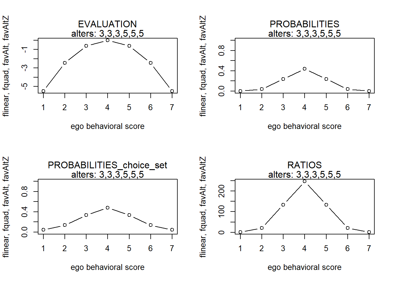
#>   x          s           p         p2         r
#> 1 1 -5.5102041 0.001785903 0.04473535   1.00000
#> 2 2 -2.4489796 0.038135608 0.13655900  21.35369
#> 3 3 -0.6122449 0.239339522 0.33290007 134.01600
#> 4 4  0.0000000 0.441477933 0.47978545 247.20157
#> 5 5 -0.6122449 0.239339522 0.33290007 134.01600
#> 6 6 -2.4489796 0.038135608 0.13655900  21.35369
#> 7 7 -5.5102041 0.001785903 0.04473535   1.00000
Here, the contribution of the average of alters’ behavior values to the evaluation function is unconditional on ego’s own value; or in other words, the tendency to ‘mimic’ the mean behavior is no different for actors with high and low behavior values. To allow for this heterogeneity, we tweak \(\beta^{beh}_4\).
finfluenceplot(alters=alters, min=1, max=7, list(flinear,fquad,favAlt,favAltZ), params = c(0,0,5,1))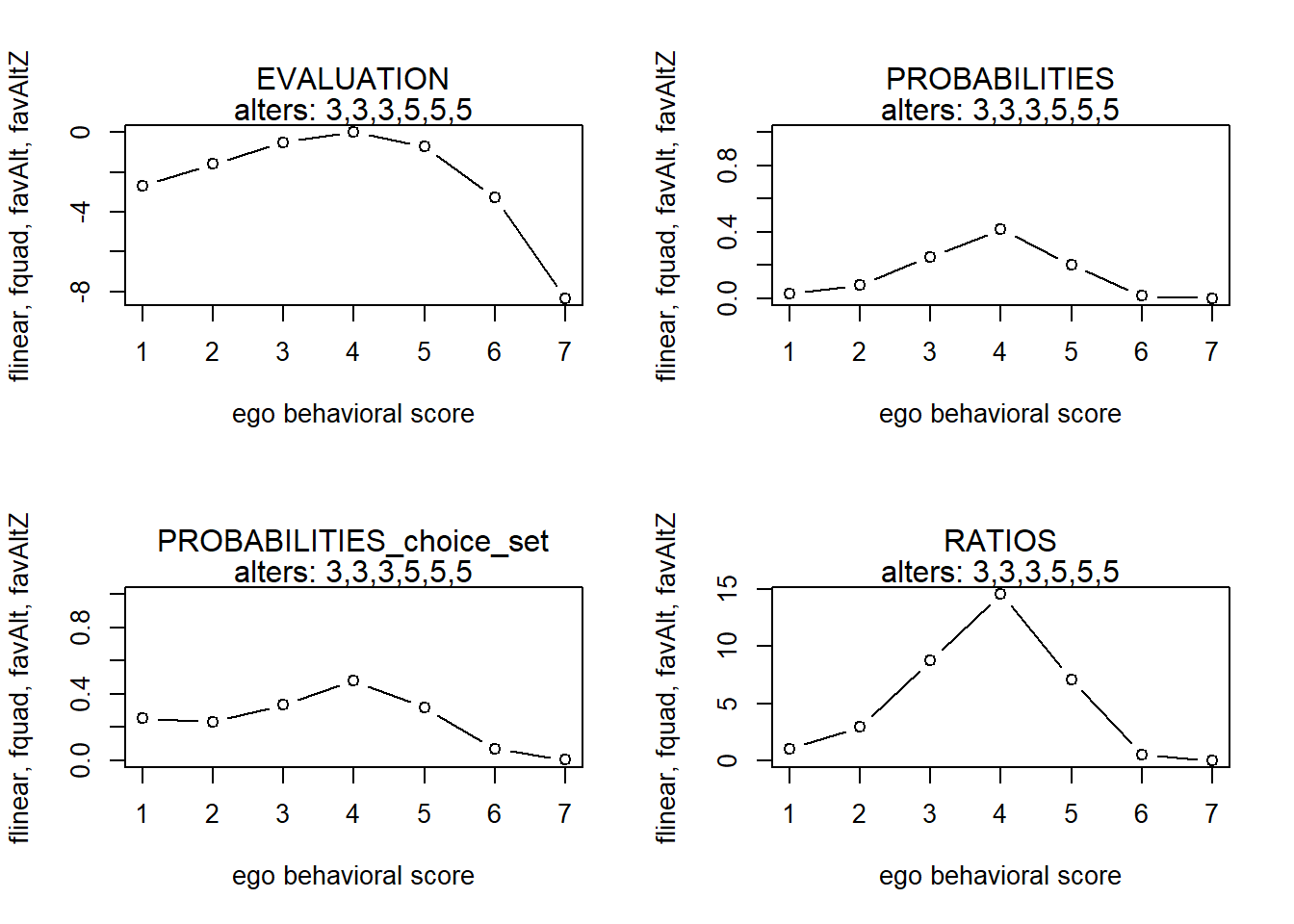
#>   x          s            p          p2            r
#> 1 1 -2.6763848 2.871190e-02 0.255963470  1.000000000
#> 2 2 -1.6093294 8.345997e-02 0.229656812  2.906807482
#> 3 3 -0.5072886 2.512398e-01 0.334115773  8.750371966
#> 4 4  0.0000000 4.172546e-01 0.478413400 14.532461039
#> 5 5 -0.7172012 2.036688e-01 0.319987966  7.093534061
#> 6 6 -3.2886297 1.556565e-02 0.070967898  0.542132470
#> 7 7 -8.3440233 9.922882e-05 0.006334476  0.003456017
finfluenceplot(alters=alters, min=1, max=7, list(flinear,fquad,favAlt,favAltZ), params = c(0,0,5,-1))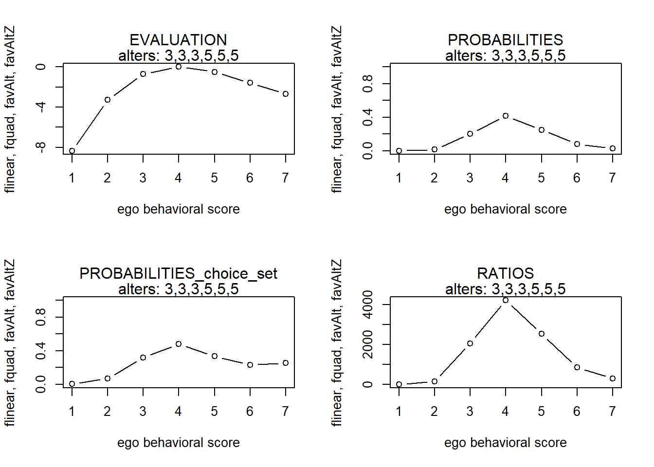
#>   x          s            p          p2         r
#> 1 1 -8.3440233 9.922882e-05 0.006334476    1.0000
#> 2 2 -3.2886297 1.556565e-02 0.070967898  156.8663
#> 3 3 -0.7172012 2.036688e-01 0.319987966 2052.5171
#> 4 4  0.0000000 4.172546e-01 0.478413400 4204.9737
#> 5 5 -0.5072886 2.512398e-01 0.334115773 2531.9238
#> 6 6 -1.6093294 8.345997e-02 0.229656812  841.0860
#> 7 7 -2.6763848 2.871190e-02 0.255963470  289.3504
This seems alright!
Many predefined RSiena effects (like the average alter effect) have the form of a product \(s^{beh}_{ik} (x,z) = z_i s^0_{ik} (x,z)\), where \(s^0_{ik} (x,z)\) does not depend on \(z_i\).
Here, if one is interested in how the magnitude of a particular effect (e.g., the in-degree effect on behavior) depends on ego’s current behavior value, one could simply interact it with the linear shape effect, like we just did.
average similarity effect
However, (average) similarity and attraction effects do not have same product-form; statistic s depends on \(z_i\) (in addition to \(z_j\), for other actors j).
If we model the average similarity effect, in interaction with the linear shape, the objective function is
\[f_i^{beh}(x,z) = \beta^{beh}_1 z_i + \beta^{beh}_2 z_i^2 + \beta^{beh}_3 x^{-1}_{i+}\sum_j x_{ij}(sim^z_{ij} - \widehat{sim^z}) + \beta^{beh}_4 z_i x^{-1}_{i+}\sum_j x_{ij}(sim^z_{ij} - \widehat{sim^z}) \]
no interaction
alters <- c(4,4,4,4,4)
finfluenceplot(alters=alters, min=1, max=7, list(flinear,fquad,favSim,favSimZ), params = c(0,0,5,0))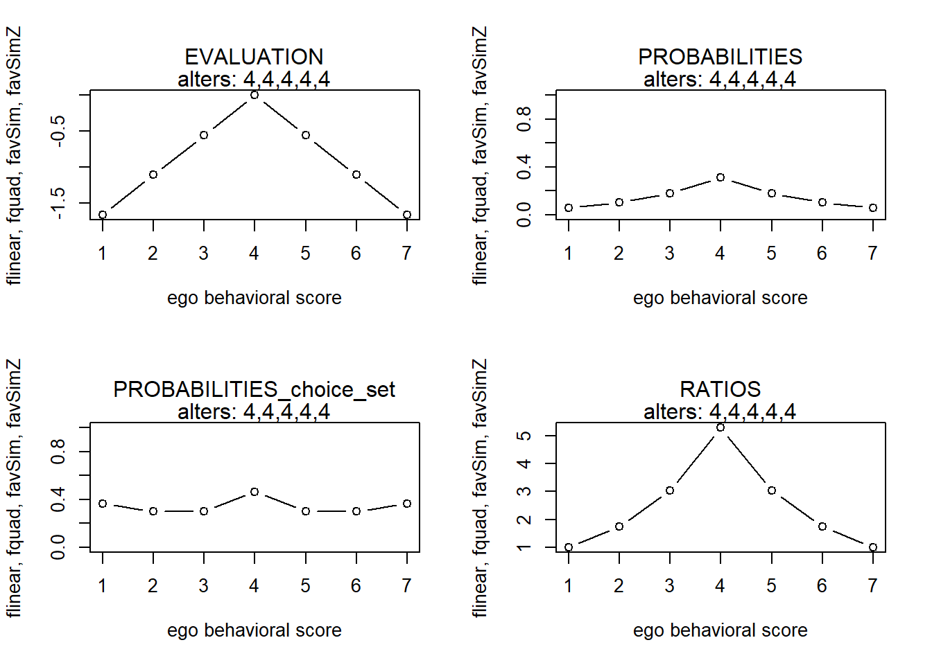
#>   x          s          p        p2        r
#> 1 1 -1.6666667 0.05932686 0.3645764 1.000000
#> 2 2 -1.1111111 0.10340132 0.3015079 1.742909
#> 3 3 -0.5555556 0.18021909 0.3015079 3.037732
#> 4 4  0.0000000 0.31410547 0.4656563 5.294490
#> 5 5 -0.5555556 0.18021909 0.3015079 3.037732
#> 6 6 -1.1111111 0.10340132 0.3015079 1.742909
#> 7 7 -1.6666667 0.05932686 0.3645764 1.000000
positive and negative interactions
finfluenceplot(alters=alters, min=1, max=7, list(flinear,fquad,favSim,favSimZ), params = c(0,0,5,.5))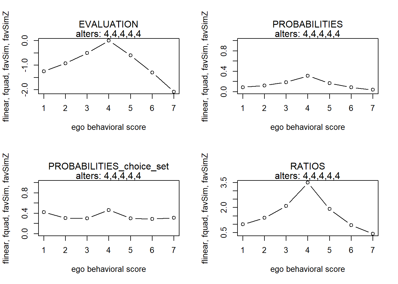
finfluenceplot(alters=alters, min=1, max=7, list(flinear,fquad,favSim,favSimZ), params = c(0,0,5,1))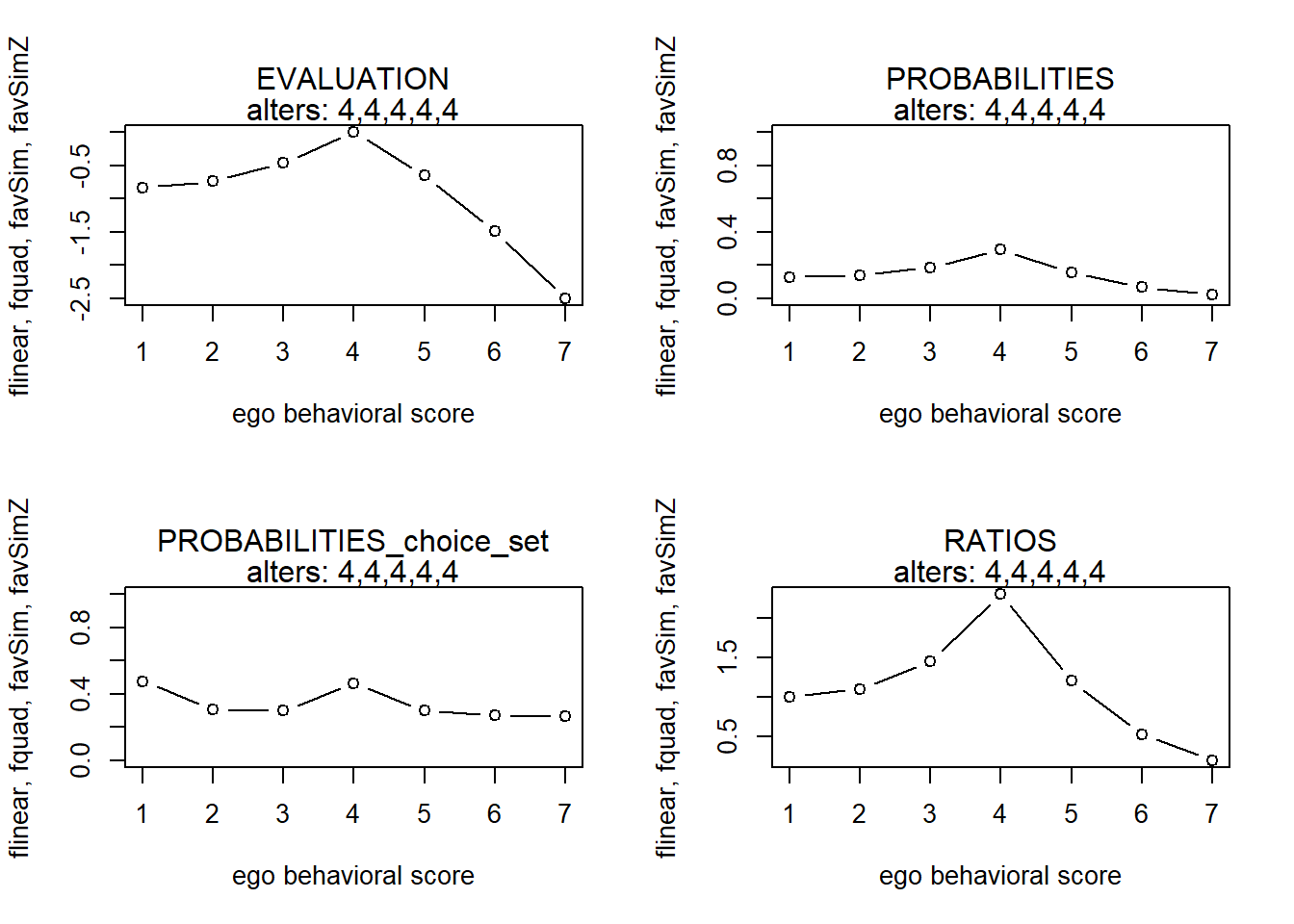
finfluenceplot(alters=alters, min=1, max=7, list(flinear,fquad,favSim,favSimZ), params = c(.5,-.1,5,1))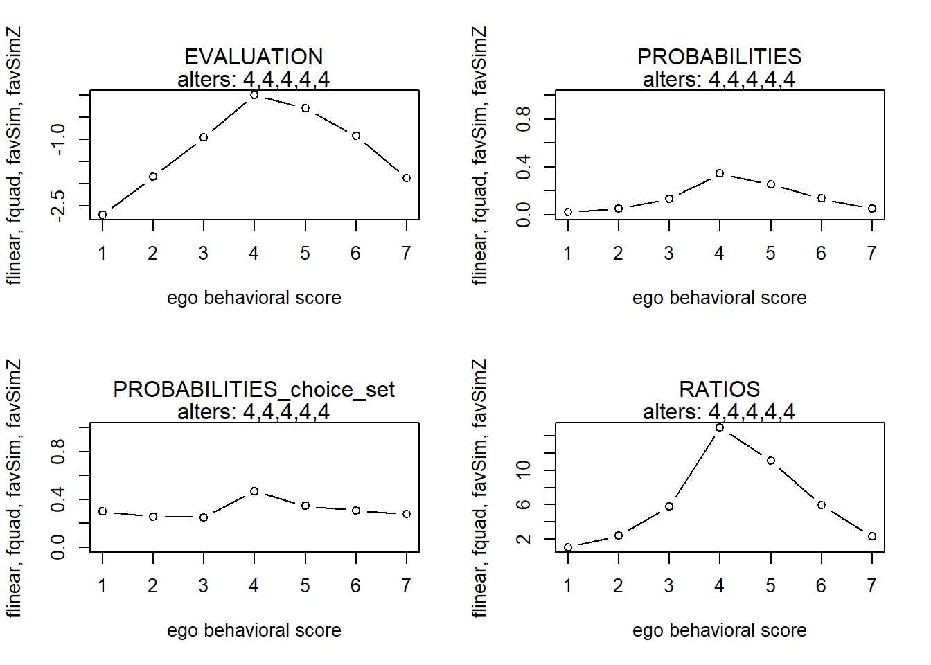
finfluenceplot(alters=alters, min=1, max=7, list(flinear,fquad,favSim,favSimZ), params = c(0,0,5,2))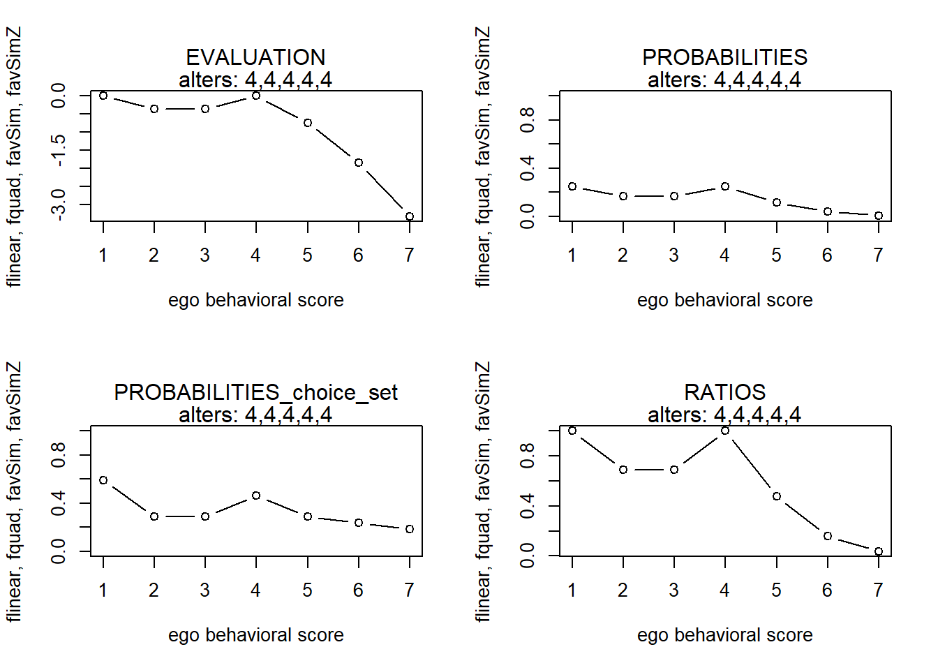
finfluenceplot(alters=alters, min=1, max=7, list(flinear,fquad,favSim,favSimZ), params = c(0,0,5,3))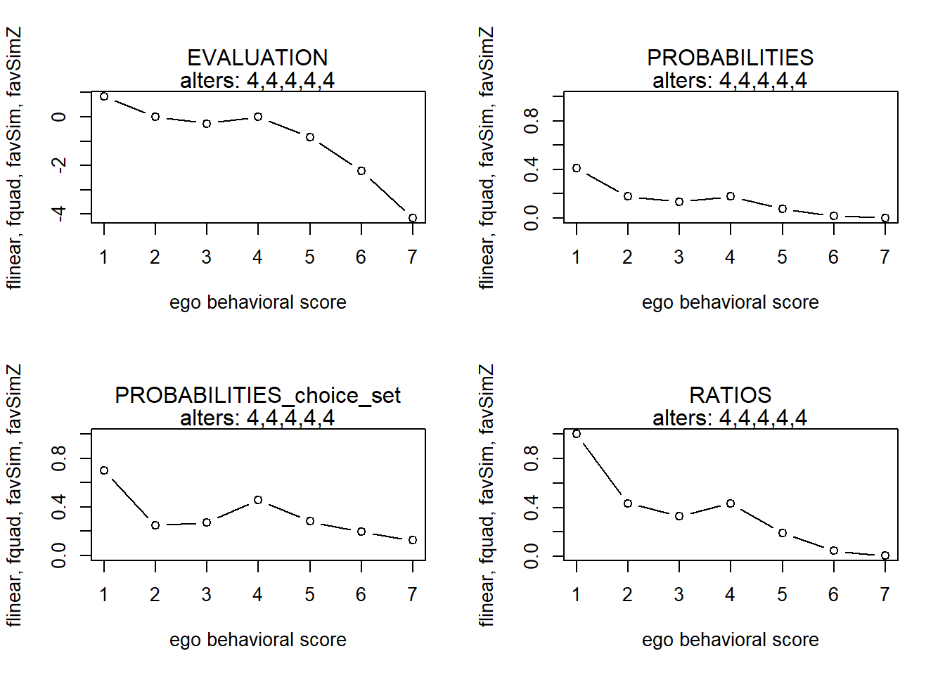
finfluenceplot(alters=alters, min=1, max=7, list(flinear,fquad,favSim,favSimZ), params = c(0,0,5,4))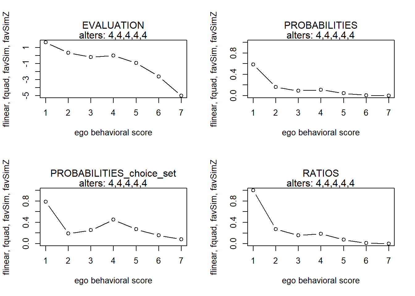
#>   x          s          p        p2         r
#> 1 1 -1.2500000 0.08871591 0.4196832 1.0000000
#> 2 2 -0.9259259 0.12267190 0.3086331 1.3827497
#> 3 3 -0.5092593 0.18608061 0.3009058 2.0974886
#> 4 4  0.0000000 0.30964895 0.4653897 3.4903430
#> 5 5 -0.6018519 0.16962454 0.3007656 1.9119968
#> 6 6 -1.2962963 0.08470232 0.2892023 0.9547590
#> 7 7 -2.0833333 0.03855578 0.3128052 0.4345982
#>   x          s          p        p2         r
#> 1 1 -0.8333333 0.12883955 0.4768684 1.0000000
#> 2 2 -0.7407407 0.14133888 0.3094291 1.0970147
#> 3 3 -0.4629630 0.18659457 0.2988429 1.4482709
#> 4 4  0.0000000 0.29645670 0.4645913 2.3009759
#> 5 5 -0.6481481 0.15505083 0.2988112 1.2034413
#> 6 6 -1.4814815 0.06738481 0.2730670 0.5230134
#> 7 7 -2.5000000 0.02433465 0.2653161 0.1888756
#>   x          s          p        p2         r
#> 1 1 -2.7083333 0.02297926 0.2980750  1.000000
#> 2 2 -1.8518519 0.05411295 0.2569968  2.354860
#> 3 3 -0.9490741 0.13346662 0.2507046  5.808133
#> 4 4  0.0000000 0.34478653 0.4700945 15.004248
#> 5 5 -0.3009259 0.25518775 0.3464558 11.105133
#> 6 6 -0.9259259 0.13659216 0.3071871  5.944149
#> 7 7 -1.8750000 0.05287473 0.2790711  2.300976
#>   x          s           p        p2          r
#> 1 1  0.0000000 0.246892977 0.5915485 1.00000000
#> 2 2 -0.3703704 0.170474305 0.2900004 0.69047855
#> 3 3 -0.3703704 0.170474305 0.2900004 0.69047855
#> 4 4  0.0000000 0.246892977 0.4614165 1.00000000
#> 5 5 -0.7407407 0.117708851 0.2918275 0.47676063
#> 6 6 -1.8518519 0.038748928 0.2344648 0.15694626
#> 7 7 -3.3333333 0.008807658 0.1852038 0.03567399
#>   x          s          p        p2           r
#> 1 1  0.8333333 0.40965147 0.6970593 1.000000000
#> 2 2  0.0000000 0.17803379 0.2464000 0.434598209
#> 3 3 -0.2777778 0.13485439 0.2746962 0.329192988
#> 4 4  0.0000000 0.17803379 0.4561912 0.434598209
#> 5 5 -0.8333333 0.07737317 0.2816641 0.188875603
#> 6 6 -2.2222222 0.01929317 0.1940445 0.047096549
#> 7 7 -4.1666667 0.00276021 0.1251604 0.006737947
#>   x          s            p         p2           r
#> 1 1  1.6666667 0.5849334833 0.78521100 1.000000000
#> 2 2  0.3703704 0.1600044841 0.19122341 0.273543042
#> 3 3 -0.1851852 0.0918031201 0.25339869 0.156946256
#> 4 4  0.0000000 0.1104796643 0.44901143 0.188875603
#> 5 5 -0.9259259 0.0437681133 0.26931819 0.074825796
#> 6 6 -2.5925926 0.0082667288 0.15662839 0.014132767
#> 7 7 -5.0000000 0.0007444061 0.08260959 0.001272634
finfluenceplot(alters=alters, min=1, max=7, list(flinear,fquad,favSim,favSimZ), params = c(0,0,5,-.5))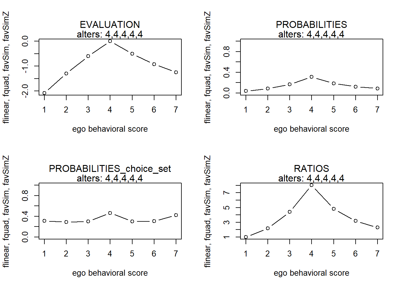
finfluenceplot(alters=alters, min=1, max=7, list(flinear,fquad,favSim,favSimZ), params = c(0,0,5,-1))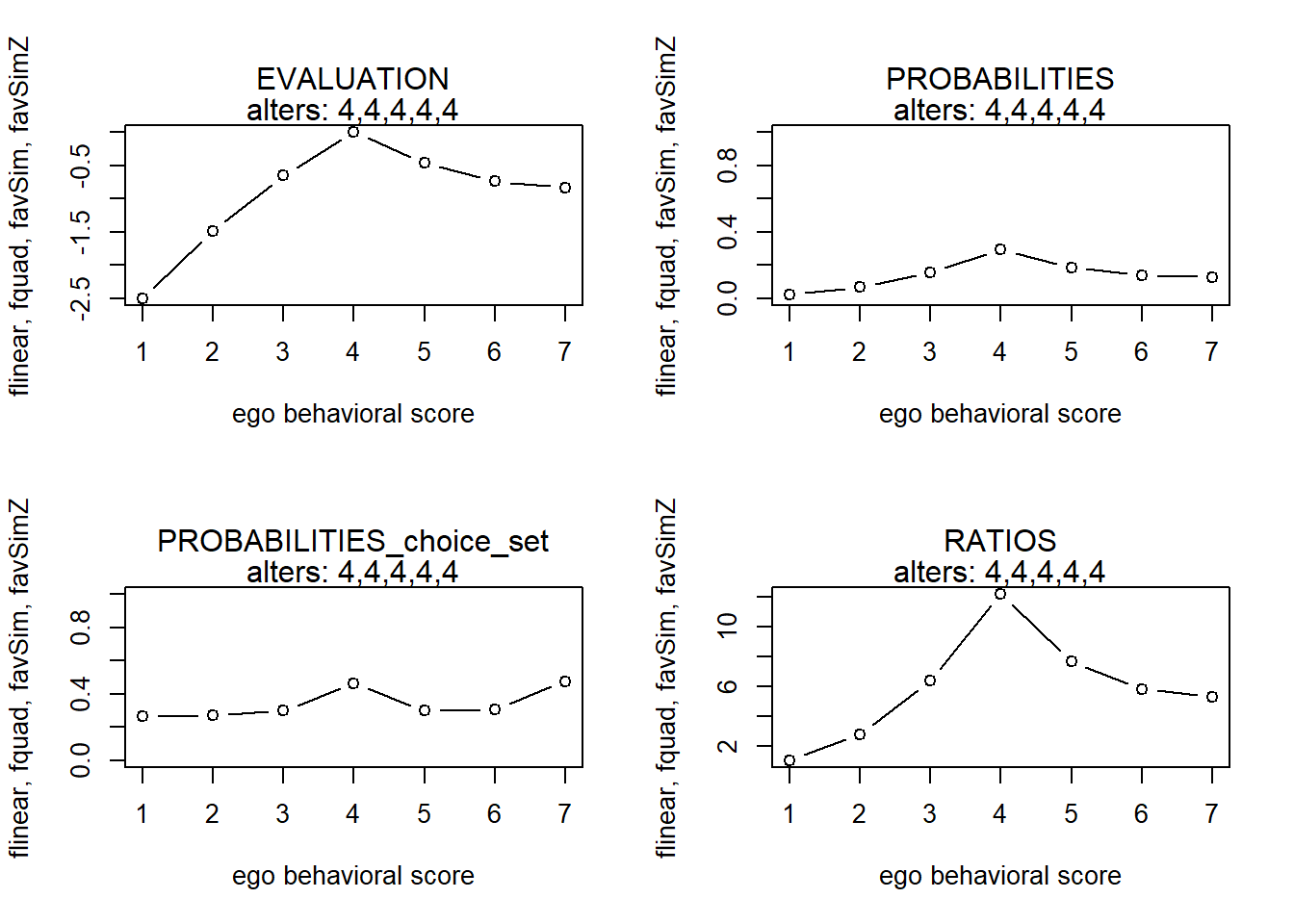
finfluenceplot(alters=alters, min=1, max=7, list(flinear,fquad,favSim,favSimZ), params = c(.5,-.1,5,-1))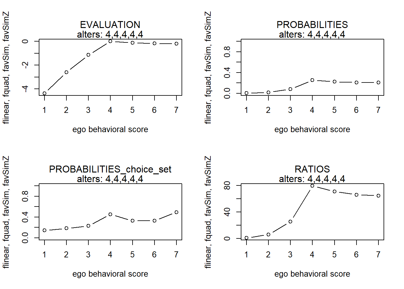
finfluenceplot(alters=alters, min=1, max=7, list(flinear,fquad,favSim,favSimZ), params = c(0,0,5,-2))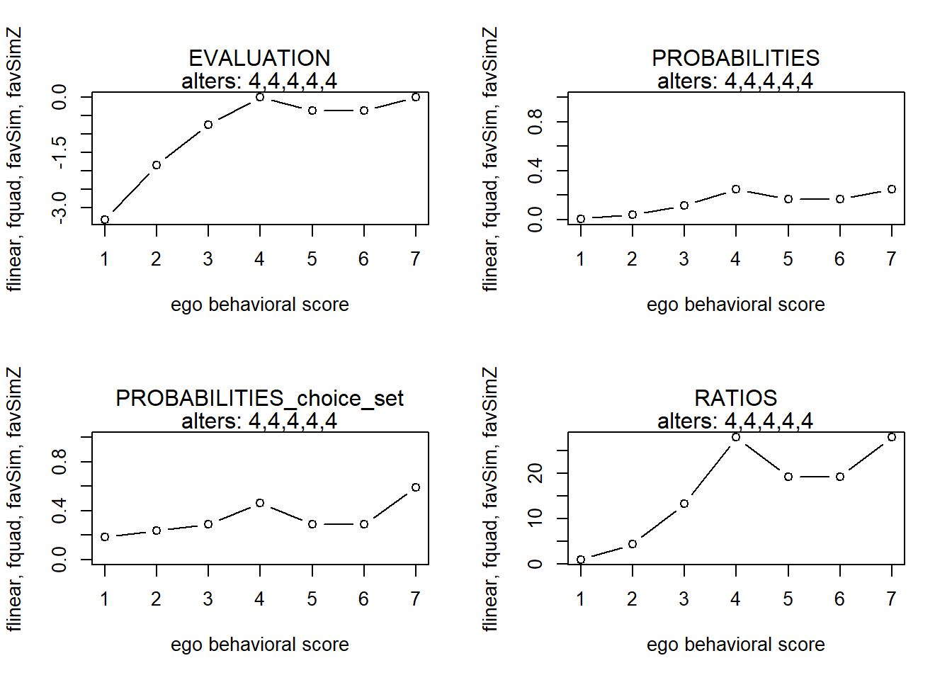
finfluenceplot(alters=alters, min=1, max=7, list(flinear,fquad,favSim,favSimZ), params = c(0,0,5,-3))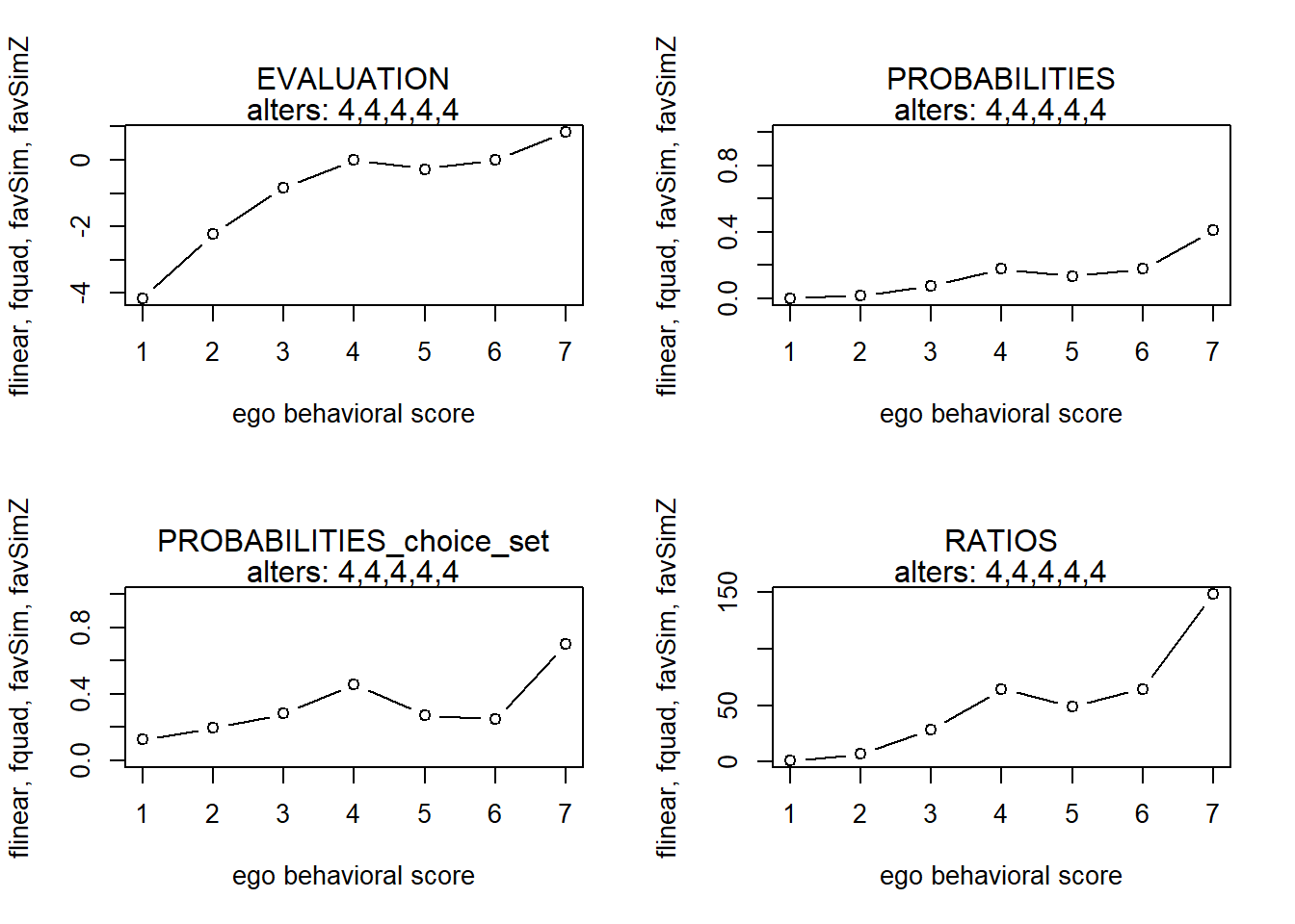
finfluenceplot(alters=alters, min=1, max=7, list(flinear,fquad,favSim,favSimZ), params = c(0,0,5,-4))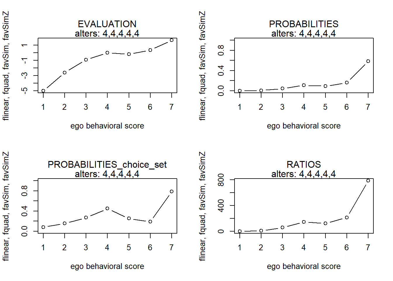
#>   x          s          p        p2        r
#> 1 1 -2.0833333 0.03855578 0.3128052 1.000000
#> 2 2 -1.2962963 0.08470232 0.2892023 2.196878
#> 3 3 -0.6018519 0.16962454 0.3007656 4.399459
#> 4 4  0.0000000 0.30964895 0.4653897 8.031195
#> 5 5 -0.5092593 0.18608061 0.3009058 4.826271
#> 6 6 -0.9259259 0.12267190 0.3086331 3.181674
#> 7 7 -1.2500000 0.08871591 0.4196832 2.300976
#>   x          s          p        p2         r
#> 1 1 -2.5000000 0.02433465 0.2653161  1.000000
#> 2 2 -1.4814815 0.06738481 0.2730670  2.769089
#> 3 3 -0.6481481 0.15505083 0.2988112  6.371608
#> 4 4  0.0000000 0.29645670 0.4645913 12.182494
#> 5 5 -0.4629630 0.18659457 0.2988429  7.667856
#> 6 6 -0.7407407 0.14133888 0.3094291  5.808133
#> 7 7 -0.8333333 0.12883955 0.4768684  5.294490
#>   x          s           p        p2         r
#> 1 1 -4.3750000 0.003192799 0.1440061  1.000000
#> 2 2 -2.5925926 0.018978472 0.1829150  5.944149
#> 3 3 -1.1342593 0.081584443 0.2303355 25.552643
#> 4 4  0.0000000 0.253635414 0.4520047 79.439840
#> 5 5 -0.1157407 0.225914615 0.3272662 70.757551
#> 6 6 -0.1851852 0.210758446 0.3279731 66.010566
#> 7 7 -0.2083333 0.205935811 0.4942132 64.500093
#>   x          s           p        p2         r
#> 1 1 -3.3333333 0.008807658 0.1852038  1.000000
#> 2 2 -1.8518519 0.038748928 0.2344648  4.399459
#> 3 3 -0.7407407 0.117708851 0.2918275 13.364375
#> 4 4  0.0000000 0.246892977 0.4614165 28.031625
#> 5 5 -0.3703704 0.170474305 0.2900004 19.355236
#> 6 6 -0.3703704 0.170474305 0.2900004 19.355236
#> 7 7  0.0000000 0.246892977 0.5915485 28.031625
#>   x             s          p        p2          r
#> 1 1 -4.166667e+00 0.00276021 0.1251604   1.000000
#> 2 2 -2.222222e+00 0.01929317 0.1940445   6.989748
#> 3 3 -8.333333e-01 0.07737317 0.2816641  28.031625
#> 4 4  0.000000e+00 0.17803379 0.4561912  64.500093
#> 5 5 -2.777778e-01 0.13485439 0.2746962  48.856571
#> 6 6  2.220446e-16 0.17803379 0.2464000  64.500093
#> 7 7  8.333333e-01 0.40965147 0.6970593 148.413159
#>   x          s            p         p2         r
#> 1 1 -5.0000000 0.0007444061 0.08260959   1.00000
#> 2 2 -2.5925926 0.0082667288 0.15662839  11.10513
#> 3 3 -0.9259259 0.0437681133 0.26931819  58.79601
#> 4 4  0.0000000 0.1104796643 0.44901143 148.41316
#> 5 5 -0.1851852 0.0918031201 0.25339869 123.32397
#> 6 6  0.3703704 0.1600044841 0.19122341 214.94246
#> 7 7  1.6666667 0.5849334833 0.78521100 785.77199
Only makes sense with low parameter values for the interaction effect!!!
average attraction (towards lower)
If we model the attraction effects, in interaction with the linear shape, the objective function is
\[f_i^{beh}(x,z) = \beta^{beh}_1 z_i + \beta^{beh}_2 z_i^2 + \beta^{beh}_3 x^{-1}_{i+}\sum_j x_{ij} (\, I \{ (z_j)<z_i \} sim^z_{ij} + I \{ (z_j ) \ge z_i \} ) + \beta^{beh}_4 z_i x^{-1}_{i+}\sum_j x_{ij} (\, I \{ (z_j)<z_i \} sim^z_{ij} + I \{ (z_j ) \ge z_i \} )\]
no interaction
finfluenceplot(alters=alters, min=1, max=7, list(flinear,fquad,favAttHigher,favAttLower,favAttLowerZ), params = c(0,0,0,5,0))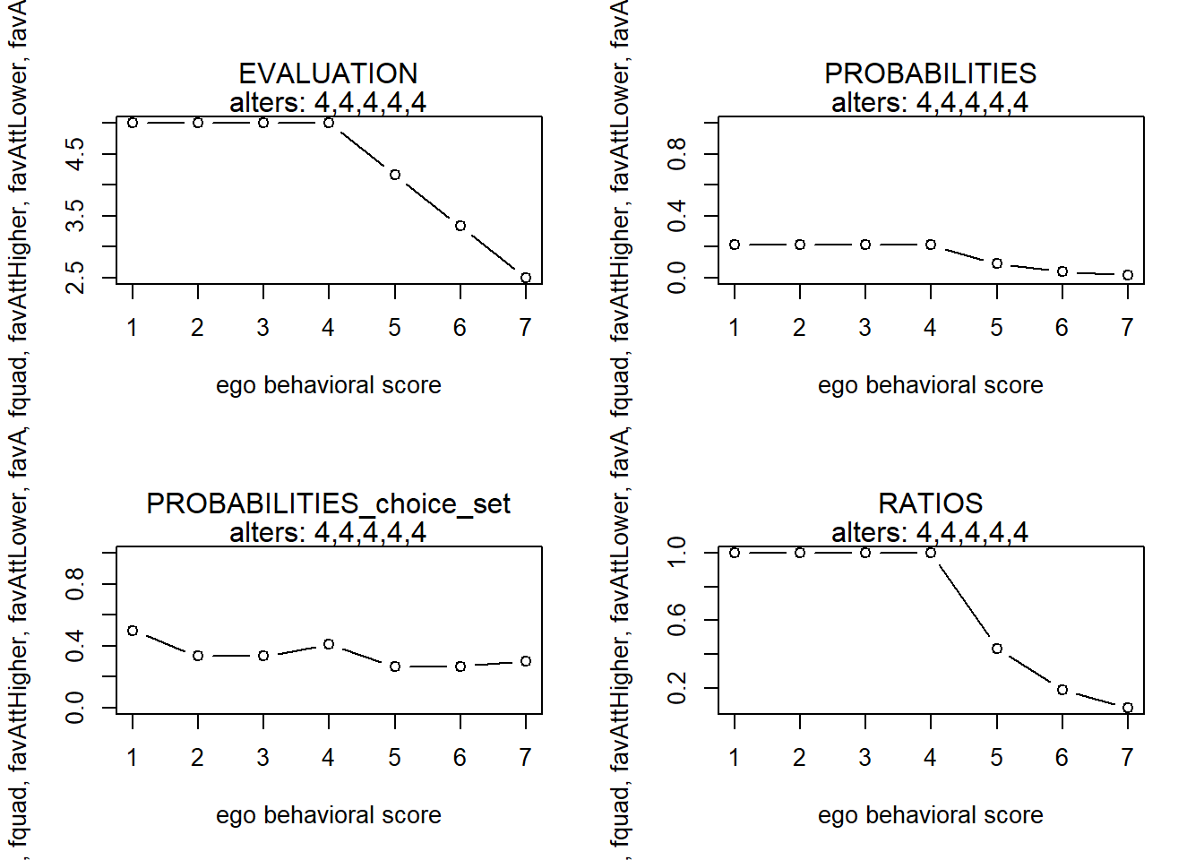
finfluenceplot(alters=alters, min=1, max=7, list(flinear,fquad,favAttHigher,favAttLower,favAttLowerZ), params = c(0,0,1,5,0))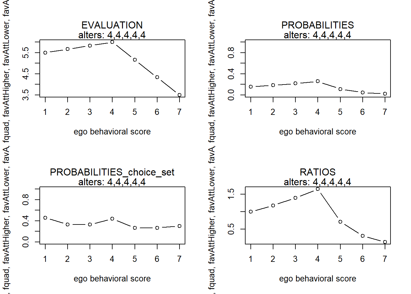
#>   x        s          p        p2         r
#> 1 1 5.000000 0.21251461 0.5000000 1.0000000
#> 2 2 5.000000 0.21251461 0.3333333 1.0000000
#> 3 3 5.000000 0.21251461 0.3333333 1.0000000
#> 4 4 5.000000 0.21251461 0.4107454 1.0000000
#> 5 5 4.166667 0.09235847 0.2676965 0.4345982
#> 6 6 3.333333 0.04013883 0.2676965 0.1888756
#> 7 7 2.500000 0.01744426 0.3029407 0.0820850
#>   x        s          p        p2         r
#> 1 1 5.500000 0.15651990 0.4584295 1.0000000
#> 2 2 5.666667 0.18490641 0.3302682 1.1813604
#> 3 3 5.833333 0.21844112 0.3302682 1.3956124
#> 4 4 6.000000 0.25805769 0.4383888 1.6487213
#> 5 5 5.166667 0.11215141 0.2676965 0.7165313
#> 6 6 4.333333 0.04874080 0.2676965 0.3114032
#> 7 7 3.500000 0.02118267 0.3029407 0.1353353
positive and negative interactions
alters <- c(2,2,2,3,3,3,3)
finfluenceplot(alters=alters, min=1, max=7, list(flinear,fquad,favAttLower,favAttLowerZ), params = c(0,0,5,0))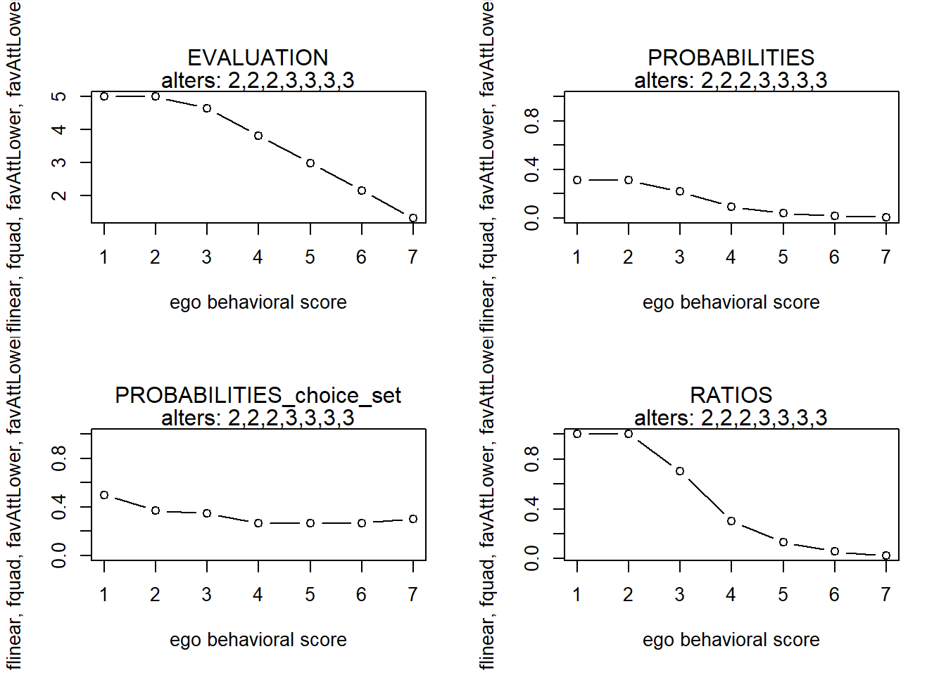
finfluenceplot(alters=alters, min=1, max=7, list(flinear,fquad,favAttLower,favAttLowerZ), params = c(0,0,5,.5))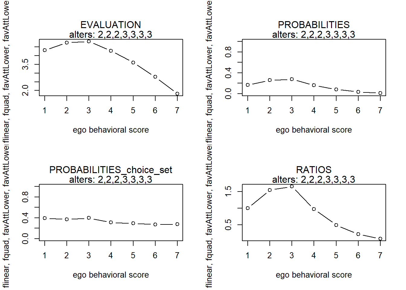
finfluenceplot(alters=alters, min=1, max=7, list(flinear,fquad,favAttLower,favAttLowerZ), params = c(0,0,5,1))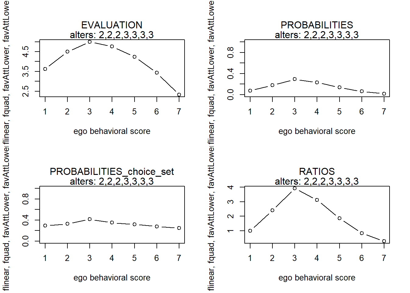
finfluenceplot(alters=alters, min=1, max=7, list(flinear,fquad,favAttLower,favAttLowerZ), params = c(0,0,5,-.5))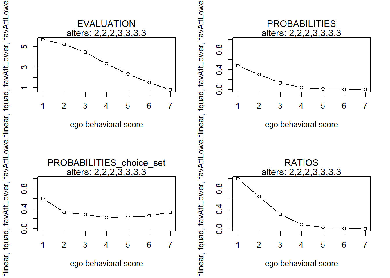
finfluenceplot(alters=alters, min=1, max=7, list(flinear,fquad,favAttLower,favAttLowerZ), params = c(0,0,5,-1))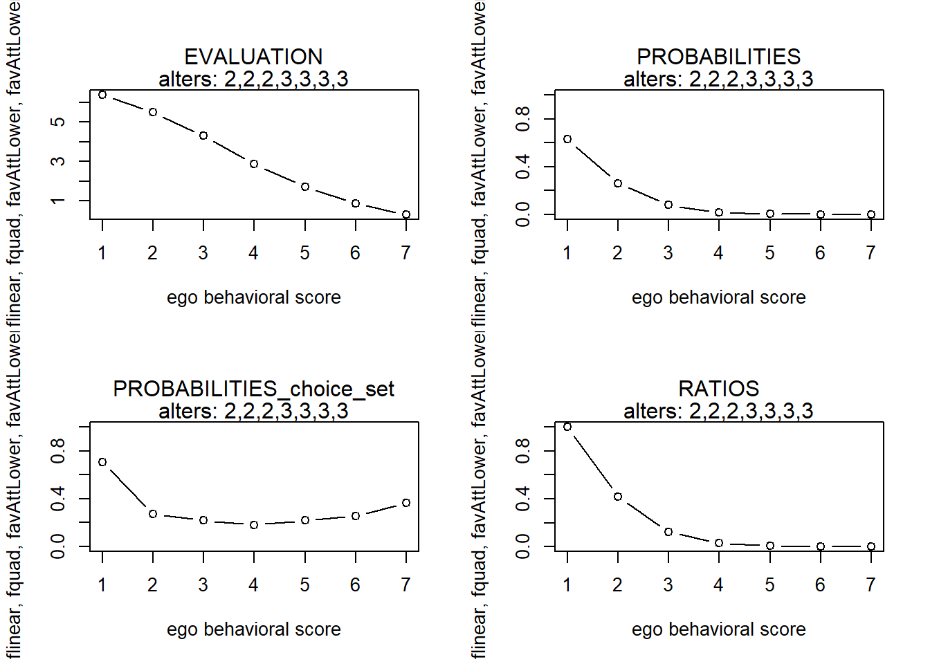
finfluenceplot(alters=alters, min=1, max=7, list(flinear,fquad,favAttLower,favAttLowerZ), params = c(0,0,5,-2))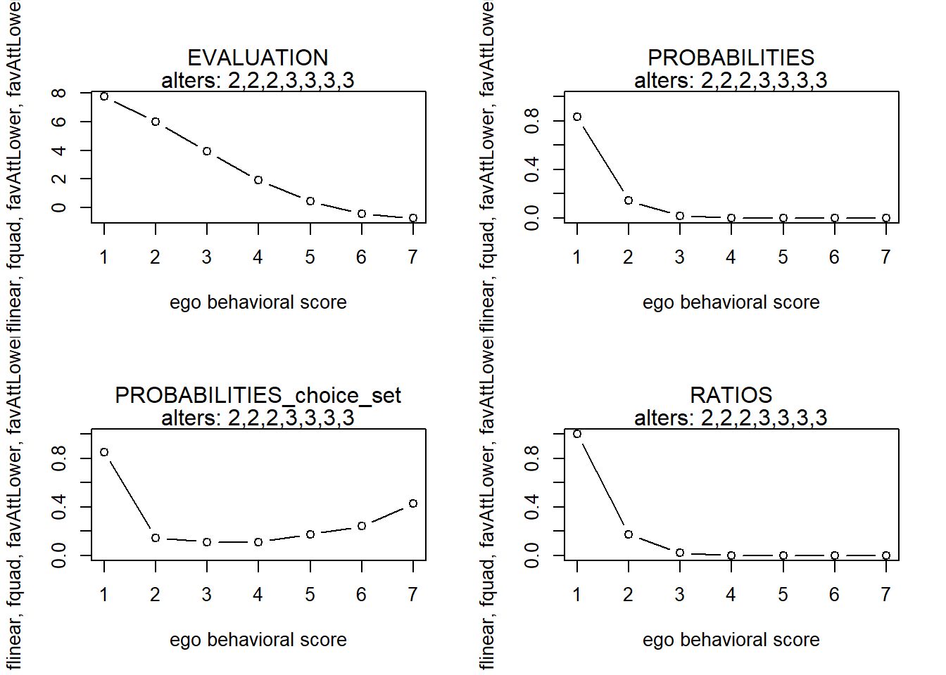
#>   x        s          p        p2          r
#> 1 1 5.000000 0.31072375 0.5000000 1.00000000
#> 2 2 5.000000 0.31072375 0.3704153 1.00000000
#> 3 3 4.642857 0.21740487 0.3491817 0.69967254
#> 4 4 3.809524 0.09448377 0.2676965 0.30407643
#> 5 5 2.976190 0.04106248 0.2676965 0.13215107
#> 6 6 2.142857 0.01784568 0.2676965 0.05743262
#> 7 7 1.309524 0.00775570 0.3029407 0.02496011
#>   x        s          p        p2          r
#> 1 1 4.312500 0.16742423 0.3923368 1.00000000
#> 2 2 4.750000 0.25931173 0.3683369 1.54883030
#> 3 3 4.816964 0.27727095 0.3963381 1.65609809
#> 4 4 4.285714 0.16299918 0.3116086 0.97356984
#> 5 5 3.608631 0.08281936 0.2934894 0.49466770
#> 6 6 2.785714 0.03637003 0.2734714 0.21723279
#> 7 7 1.816964 0.01380451 0.2751297 0.08245227
#>   x        s          p        p2         r
#> 1 1 3.625000 0.07472965 0.2942150 1.0000000
#> 2 2 4.500000 0.17926710 0.3277691 2.3988753
#> 3 3 4.991071 0.29293428 0.4154262 3.9199207
#> 4 4 4.761905 0.23294017 0.3506832 3.1171052
#> 5 5 4.241071 0.13837236 0.3197772 1.8516394
#> 6 6 3.428571 0.06140236 0.2789383 0.8216600
#> 7 7 2.324405 0.02035409 0.2489600 0.2723696
#>   x         s           p        p2           r
#> 1 1 5.6875000 0.477494475 0.6076632 1.000000000
#> 2 2 5.2500000 0.308293604 0.3325946 0.645648526
#> 3 3 4.4687500 0.141147097 0.2852669 0.295599435
#> 4 4 3.3333333 0.045348900 0.2230051 0.094972617
#> 5 5 2.3437500 0.016857617 0.2427062 0.035304318
#> 6 6 1.5000000 0.007250371 0.2615959 0.015184198
#> 7 7 0.8020833 0.003607936 0.3322743 0.007555975
#>   x         s           p        p2           r
#> 1 1 6.3750000 0.630062575 0.7057850 1.000000000
#> 2 2 5.5000000 0.262649157 0.2703828 0.416862020
#> 3 3 4.2946429 0.078685744 0.2185567 0.124885602
#> 4 4 2.8571429 0.018689502 0.1808935 0.029662931
#> 5 5 1.7113095 0.005942493 0.2187849 0.009431591
#> 6 6 0.8571429 0.002529349 0.2551542 0.004014441
#> 7 7 0.2946429 0.001441180 0.3629692 0.002287360
#>   x          s            p        p2            r
#> 1 1  7.7500000 0.8332486504 0.8519528 1.0000000000
#> 2 2  6.0000000 0.1447969039 0.1452880 0.1737739435
#> 3 3  3.9464286 0.0185739613 0.1120385 0.0222910187
#> 4 4  1.9047619 0.0024111263 0.1119061 0.0028936457
#> 5 5  0.4464286 0.0005608850 0.1749582 0.0006731304
#> 6 6 -0.4285714 0.0002338117 0.2412026 0.0002806025
#> 7 7 -0.7202381 0.0001746614 0.4275959 0.0002096150
Hmmm… this is not what I want! Ego should not be drawn up by higher alters in the case of a positive attraction towards lower parameter; ego should not move away from higher alters in the case of a negative parameter. That’s exactly why the similarity scores for alters who did not score lower than ego were replaced by 1. Thus, alters that are (no longer) lower than me, have no influence anymore. But since the average similarity of alters is now multiplied by ego’s own behavior, ego will always prefer increasing the behavior over staying constant (at least, in the case of a postive paramter for the interaction effect.
Copyright © 2021 Rob Franken